Chapter 1 The Big (Bayesian) Picture

How can we live if we don’t change?
—Beyoncé. Lyric from “Satellites.”

Everybody changes their mind. You likely even changed your mind in the last minute. Prior to ever opening it, you no doubt had some preconceptions about this book, whether formed from its title, its online reviews, or a conversation with a friend who has read it. And then you saw that the first chapter opened with a quote from Beyoncé, an unusual choice for a statistics book. Perhaps this made you think “This book is going to be even more fun than I realized!” Perhaps it served to do the opposite. No matter. The point we want to make is that we agree with Beyoncé – changing is simply part of life.

We continuously update our knowledge about the world as we accumulate lived experiences, or collect data. As children, it takes a few spills to understand that liquid doesn’t stay in a glass. Or a couple attempts at conversation to understand that, unlike in cartoons, real dogs can’t talk. Other knowledge is longer in the making. For example, suppose there’s a new Italian restaurant in your town. It has a 5-star online rating and you love Italian food! Thus, prior to ever stepping foot in the restaurant, you anticipate that it will be quite delicious. On your first visit, you collect some edible data: your pasta dish arrives a soggy mess. Weighing the stellar online rating against your own terrible meal (which might have just been a fluke), you update your knowledge: this is a 3-star not 5-star restaurant. Willing to give the restaurant another chance, you make a second trip. On this visit, you’re pleased with your Alfredo and increase the restaurant’s rating to 4 stars. You continue to visit the restaurant, collecting edible data and updating your knowledge each time.

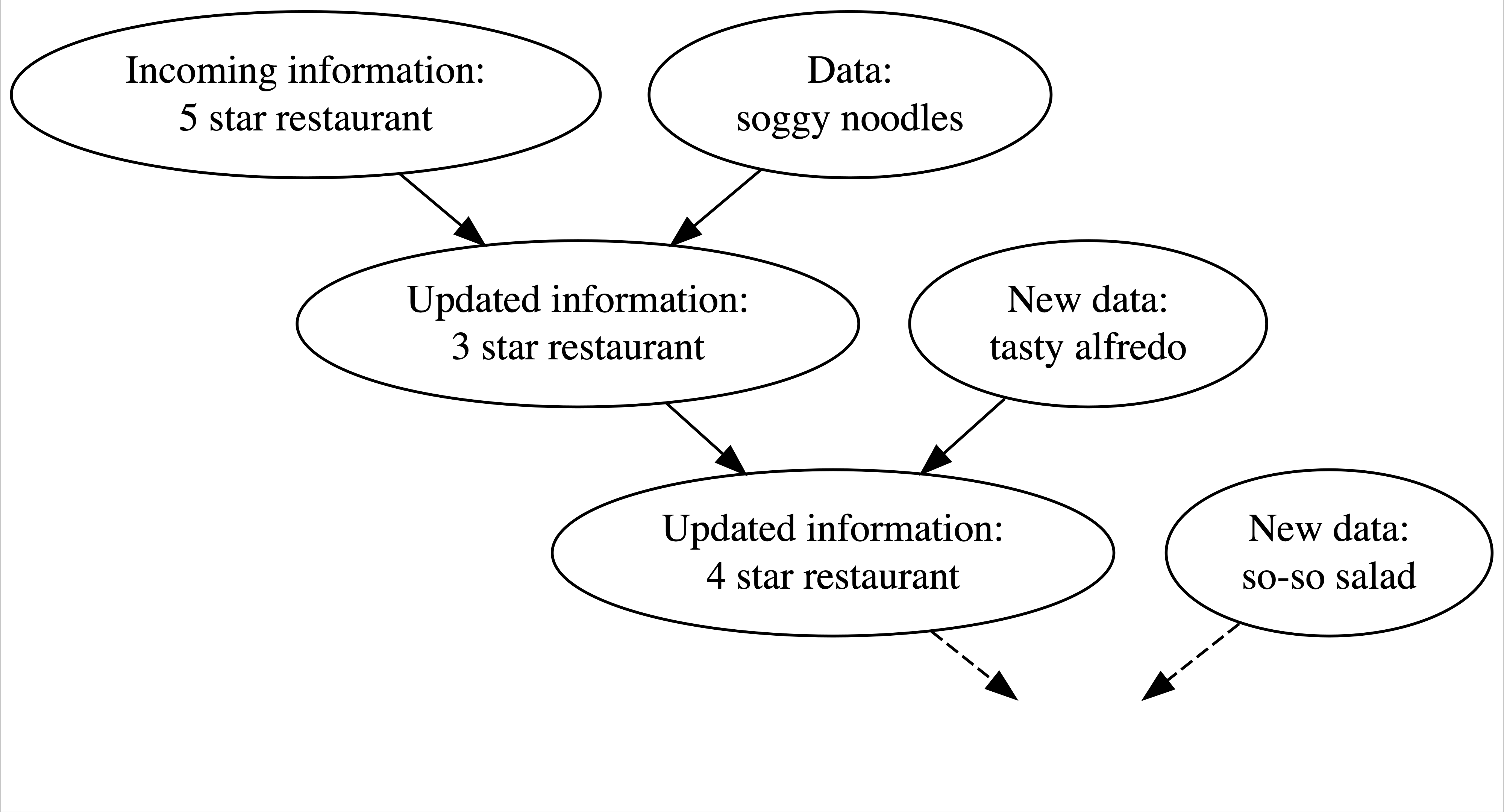
FIGURE 1.1: Your evolving knowledge about a restaurant.

Figure 1.1 captures the natural Bayesian knowledge-building process of acknowledging your preconceptions, using data to update your knowledge, and repeating. We can apply this same Bayesian process to rigorous research inquiries. If you’re a political scientist, yours might be a study of demographic factors in voting patterns. If you’re an environmental scientist, yours might be an analysis of the human role in climate change. You don’t walk into such an inquiry without context – you carry a degree of incoming or prior information based on previous research and experience. Naturally, it’s in light of this information that you interpret new data, weighing both in developing your updated or posterior information. You continue to refine this information as you gather new evidence (Figure 1.2).

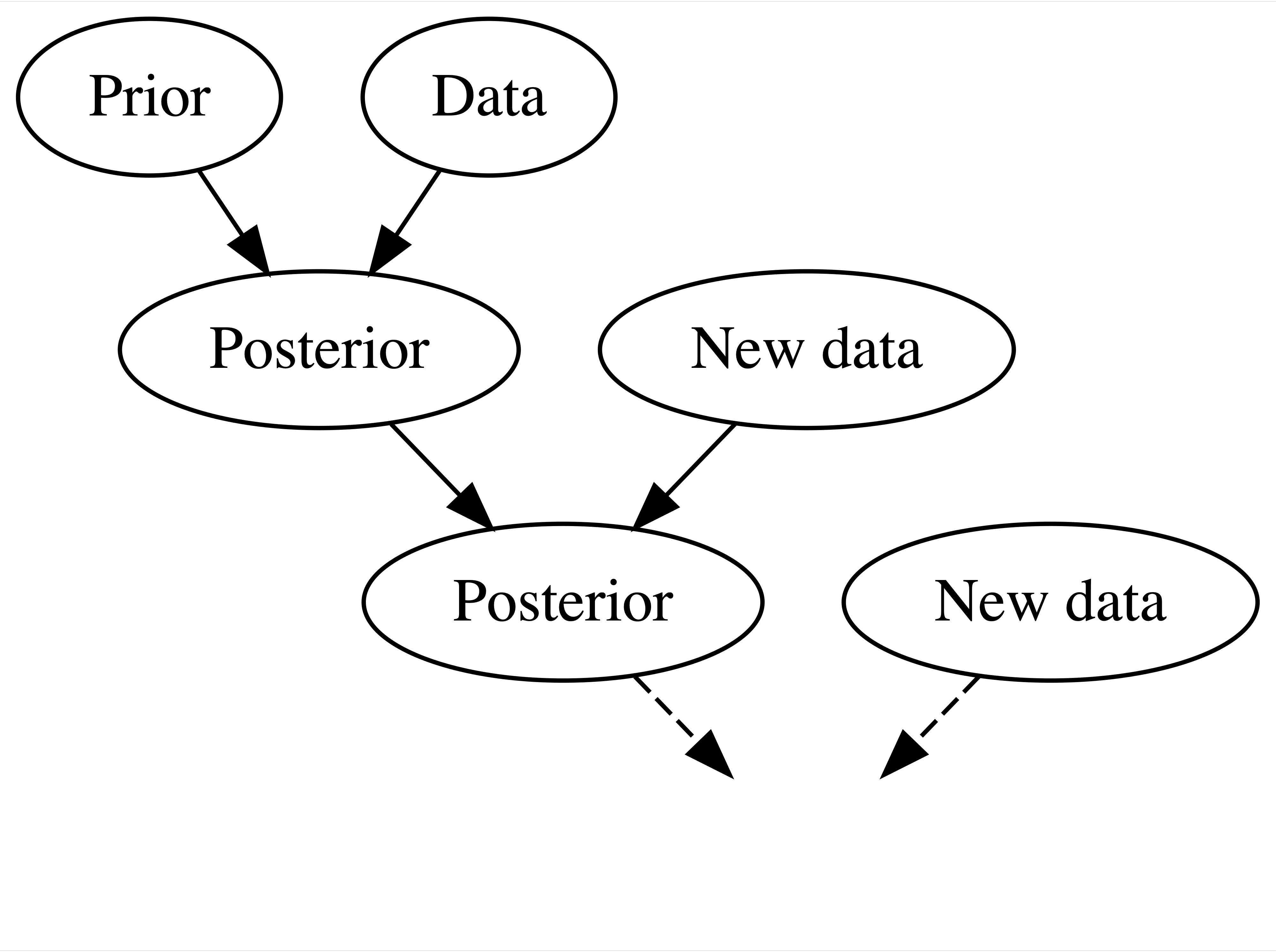
FIGURE 1.2: A Bayesian knowledge-building diagram.

The Bayesian philosophy represented in Figure 1.2 is the foundation of Bayesian statistics. Throughout this book, you will build the methodology and tools you need to implement this philosophy in a rigorous data analysis. This experience will require a sense of purpose and a map.

• Learn to think like a Bayesian.
• Explore the foundations of a Bayesian data analysis and how they contrast with the frequentist alternative.
• Learn a little bit about the history of the Bayesian philosophy.

1.1 Thinking like a Bayesian

Given our emphasis on how natural the Bayesian approach to knowledge-building is, you might be surprised to know that the alternative frequentist philosophy has traditionally dominated statistics. Before exploring their differences, it’s important to note that Bayesian and frequentist analyses share a common goal: to learn from data about the world around us. Both Bayesian and frequentist analyses use data to fit models, make predictions, and evaluate hypotheses. When working with the same data, they will typically produce a similar set of conclusions. Moreover, though we’ll often refer to people applying these philosophies as “Bayesians” and “frequentists,” this is for brevity only. The distinction is not always so clear in practice – even the authors apply both philosophies in their work, and thus don’t identify with a single label. Our goal here is not to “take sides,” but to illustrate the key differences in the logic behind, approach to, and interpretation of Bayesian and frequentist analyses.

1.1.1 Quiz yourself

Before we elaborate upon the Bayesian vs frequentist philosophies, take a quick quiz to assess your current inclinations. In doing so, try to abandon any rules that you might have learned in the past and just go with your gut.

1. When flipping a fair coin, we say that “the probability of flipping Heads is 0.5.” How do you interpret this probability?

   1. If I flip this coin over and over, roughly 50% will be Heads.
   2. Heads and Tails are equally plausible.
   3. Both a and b make sense.

2. An election is coming up and a pollster claims that candidate A has a 0.9 probability of winning. How do you interpret this probability?

   1. If we observe the election over and over, candidate A will win roughly 90% of the time.
   2. Candidate A is much more likely to win than to lose.
   3. The pollster’s calculation is wrong. Candidate A will either win or lose, thus their probability of winning can only be 0 or 1.

3. Consider two claims. (1) Zuofu claims that he can predict the outcome of a coin flip. To test his claim, you flip a fair coin 10 times and he correctly predicts all 10. (2) Kavya claims that she can distinguish natural and artificial sweeteners. To test her claim, you give her 10 sweetener samples and she correctly identifies each. In light of these experiments, what do you conclude?

   1. You’re more confident in Kavya’s claim than Zuofu’s claim.
   2. The evidence supporting Zuofu’s claim is just as strong as the evidence supporting Kavya’s claim.

4. Suppose that during a recent doctor’s visit, you tested positive for a very rare disease. If you only get to ask the doctor one question, which would it be?

   1. What’s the chance that I actually have the disease?
   2. If in fact I don’t have the disease, what’s the chance that I would’ve gotten this positive test result?

Next, tally up your quiz score using the scoring system below.¹ Totals from 4–5 indicate that your current thinking is fairly frequentist, whereas totals from 9–12 indicate alignment with the Bayesian philosophy. In between these extremes, totals from 6–8 indicate that you see strengths in both philosophies. Your current inclinations might be more frequentist than Bayesian or vice versa. These inclinations might change throughout your reading of this book. They might not. For now, we merely wish to highlight the key differences between the Bayesian and frequentist philosophies.

1.1.2 The meaning of probability

Probability theory is central to every statistical analysis. Yet, as illustrated by questions 1 and 2 in Section 1.1.1, Bayesians and frequentists differ on something as fundamental as the meaning of probability. For example, in question 1, a Bayesian and frequentist would both say that the probability of observing Heads on a fair coin flip is 1/2. The difference is in their interpretation.

Interpreting probability

• In the Bayesian philosophy, a probability measures the relative plausibility of an event.
• The frequentist philosophy is so named for its interpretation of probability as the long-run relative frequency of a repeatable event.

Thus, in the coin flip example, a Bayesian would conclude that Heads and Tails are equally likely. In contrast, a frequentist would conclude that if we flip the coin over and over and over, roughly 1/2 of these flips will be Heads. Let’s try applying these same ideas to the question 2 setting in which a pollster declares that candidate A has a 0.9 probability of winning the upcoming election. This routine election calculation illustrates cracks within the frequentist interpretation. Since the election is a one-time event, the long-run relative frequency concept of observing the election over and over simply doesn’t apply. A very strict frequentist interpretation might even conclude the pollster is just wrong. Since the candidate will either win or lose, their win probability must be either 1 or 0. A less extreme frequentist interpretation, though a bit awkward, is more reasonable: in long-run hypothetical repetitions of the election, i.e., elections with similar circumstances, candidate A would win roughly 90% of the time.

The election example is not rare. It’s often the case that an event of interest is unrepeatable. Whether or not a politician wins an election, whether or not it rains tomorrow, and whether or not humans will live on Mars are all one-time events. Whereas the frequentist interpretation of probability can be awkward in these one-time settings, the more flexible Bayesian interpretation provides a path by which to express the uncertainty of these events. For example, a Bayesian would interpret “a 0.9 probability of winning” to mean that, based on election models, the relative plausibility of winning is high – the candidate is 9 times more likely to win than to lose.

1.1.3 The Bayesian balancing act

Inspired by an example by Berger (1984), question 3 in Section 1.1.1 presented you with two scenarios: (1) Zuofu claims that he can predict the outcome of a coin flip and (2) Kavya claims that she can distinguish between natural and artificial sweeteners. Let’s agree here that the first claim is simply ridiculous but that the second is plausible (some people have sensitive palates!). Thus, imagine our surprise when, in testing their claims, both Zuofu and Kavya enjoyed a 10 out of 10 success rate: Zuofu correctly predicted the outcomes of 10 coin flips and Kavya correctly identified the source of 10 different sweeteners. What can we conclude from this data? Does it provide equal evidence in support of both Zuofu’s and Kavya’s claims? The Bayesian and frequentist philosophies view these questions through different lenses.

Let’s begin by looking through the frequentist lens which, to oversimplify quite a bit, analyzes the data absent a consideration of our prior contextual understanding. Thus, in a frequentist analysis, “10 out of 10” is “10 out of 10” no matter if it’s in the context of Zuofu’s coins or Kavya’s sweeteners. This means that a frequentist analysis would lead to equally confident conclusions that Zuofu can predict coin flips and Kavya can distinguish between natural and artificial sweeteners (at least on paper if not in our gut).² Given the absurdity of Zuofu’s claim, this frequentist conclusion is a bit bizarre – it throws out all prior knowledge in favor of a mere 10 data points. We can’t resist representing this conclusion with Figure 1.3, a frequentist complement to the Bayesian knowledge-building diagram in Figure 1.2, which solely consists of the data.

FIGURE 1.3: A frequentist knowledge-building diagram.

In contrast, a Bayesian analysis gives voice to our prior knowledge. Here, our experience on Earth suggests that Zuofu is probably overstating his abilities but that Kavya’s claim is reasonable. Thus, after weighing their equivalent “10 out of 10” achievements against these different priors, our posterior understanding of Zuofu’s and Kavya’s claims differ. Since the data is consistent with our prior, we’re even more certain that Kavya is a sweetener savant. However, given its inconsistency with our prior experience, we are chalking Zuofu’s “psychic” achievement up to simple luck.

The idea of allowing one’s prior experience to play a formal role in a statistical analysis might seem a bit goofy. In fact, a common critique of the Bayesian philosophy is that it’s too subjective. We haven’t done much to combat this critique yet. Favoring flavor over details, Figure 1.2 might even lead you to believe that Bayesian analysis involves a bit of subjective hocus pocus: combine your prior with some data and poof, out pops your posterior. In reality, the Bayesian philosophy provides a formal framework for such knowledge creation. This framework depends upon prior information, data, and the balance between them.

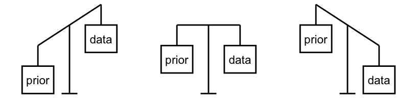
FIGURE 1.4: Bayesian analyses balance our prior experiences with new data. Depending upon the setting, the prior is given more weight than the data (left), the prior and data are given equal weight (middle), or the prior is given less weight than the data (right).

In building the posterior, the balance between the prior information and data is determined by the relative strength of each. For example, we had a very strong prior understanding that Zuofu isn’t a psychic, yet very little data (10 coin flips) supporting his claim. Thus, like the left plot in Figure 1.4, the prior held more weight in our posterior understanding. However, we’re not stubborn. If Zuofu had correctly predicted the outcome of, say, 10,000 coin flips, the strength of this data would far surpass that of our prior, leading to a posterior conclusion that perhaps Zuofu is psychic after all (like the right plot in Figure 1.4)!

Allowing the posterior to balance out the prior and data is critical to the Bayesian knowledge-building process. When we have little data, our posterior can draw upon the power in our prior knowledge. As we collect more data, the prior loses its influence. Whether in science, policy-making, or life, this is how people tend to think (El-Gamal and Grether 1995) and how progress is made. As they collect more and more data, two scientists will come to agreement on the human role in climate change, no matter their prior training and experience.³ As they read more and more pages of this book, two readers will come to agreement on the power of Bayesian statistics. This logical and heartening idea is illustrated by Figure 1.5.

FIGURE 1.5: A two-person Bayesian knowledge-building diagram.

1.1.4 Asking questions

In question 4 of Section 1.1.1, you were asked to imagine that you tested positive for a rare disease and only got to ask the doctor one question: (a) what’s the chance that I actually have the disease?, or (b) if in fact I do not have the disease, what’s the chance that I would’ve gotten this positive test result? The authors are of the opinion that, though the answers to both questions would be helpful, we’d rather know the answer to (a). That is, we’d rather understand the uncertainty in our unknown disease status than in our observed test result. Unsurprising spoiler: though Bayesian and frequentist analyses share the goal of using your test results (the data) to assess whether you have the rare disease (the hypothesis), a Bayesian analysis would answer (a) whereas a frequentist analysis would answer (b). Specifically, a Bayesian analysis assesses the uncertainty of the hypothesis in light of the observed data, and a frequentist analysis assesses the uncertainty of the observed data in light of an assumed hypothesis.

Asking questions

• A Bayesian hypothesis test seeks to answer: In light of the observed data, what’s the chance that the hypothesis is correct?
• A frequentist hypothesis test seeks to answer: If in fact the hypothesis is incorrect, what’s the chance I’d have observed this, or even more extreme, data?

For clarity, consider the scenario summarized in Table 1.1 where, in a population of 100, only four people have the disease. Among the 96 without the disease, nine test positive and thus get misleading test results. Among the four with the disease, three test positive and thus get accurate test results.

TABLE 1.1: Disease status and test outcomes for 100 people.

	test positive	test negative	total
disease	3	1	4
no disease	9	87	96
total	12	88	100

In this scenario, a Bayesian analysis would ask: Given my positive test result, what’s the chance that I actually have the disease? Since only 3 of the 12 people that tested positive have the disease (Table 1.1), there’s only a 25% chance that you have the disease. Thus, when we take into account the disease’s rarity and the relatively high false positive rate, it’s relatively unlikely that you actually have the disease. What a relief.

Recalling Section 1.1.2, you might anticipate that a frequentist approach to this analysis would differ. From the frequentist standpoint, since disease status isn’t repeatable, the probability you have the disease is either 1 or 0 – you have it or you don’t. To the contrary, medical testing (and data collection in general) is repeatable. You can get tested for the disease over and over and over. Thus, a frequentist analysis would ask: If I don’t actually have the disease, what’s the chance that I would’ve tested positive? Since only 9 of the 96 people without the disease tested positive, there’s a roughly 10% (9/96) chance that you would’ve tested positive even if you didn’t have the disease.

The 9/96 frequentist probability calculation is similar in spirit to a p-value. In general, p-values measure the chance of having observed data as or more extreme than ours if in fact our original hypothesis is incorrect. Though the p-value was prominent in the frequentist practice for decades, it’s slowly being de-emphasized across the frequentist and Bayesian spectrum. Essentially, it’s so commonly misinterpreted and misused (Goodman 2011), that the American Statistical Association put out an official “public safety announcement” regarding its usage (Wasserstein 2016). The reason the p-value is so commonly misinterpreted is simple – it’s more natural to study the uncertainty of a yet-unproven hypothesis (whether you have the rare disease) than the uncertainty of data we have already observed (you tested positive for the rare disease).⁴

1.2 A quick history lesson

Given how natural Bayesian thinking is, you might be surprised to know that Bayes’ momentum is relatively recent. Once an obscure term outside specialized industry and research circles, “Bayesian” has popped up on TV shows (e.g., The Big Bang Theory⁵ and Numb3rs⁶), has been popularized by various blogs, and regularly appears in the media (e.g., the New York Times’ explanation of how to think like an epidemiologist (Roberts 2020)).

Despite its recent rise in popularity, Bayesian statistics is rooted in the eighteenth-century work of Reverend Thomas Bayes, a statistician, minister, and philosopher. Though Bayes developed his philosophy during the 1740s, it wasn’t until the late twentieth century that this work reached a broad audience. During the more than two centuries in between, the frequentist philosophy dominated statistical research and practice. The Bayesian philosophy not only fell out of popular favor during this time, it was stigmatized. As recently as 1990, Marilyn vos Savant was ridiculed by some readers of her Parade magazine column when she presented a Bayesian solution to the now classic Monty Hall probability puzzle. Apparently more than 10,000 readers wrote in to dispute and mock her solution.⁷ Vos Savant’s Bayesian solution was later proven to be indisputably correct. Yet with this level of scrutiny, it’s no wonder that many researchers kept their Bayesian pursuits under wraps. Though neither proclaimed as much at the time, Alan Turing cracked Germany’s Enigma code in World War II and John Tukey pioneered election-day predictions in the 1960s using Bayesian methods (McGrayne 2012).

As the public existence of this book suggests, the stigma has largely eroded. Why? (1) Advances in computing. Bayesian applications require sophisticated computing resources that weren’t broadly available until the 1990s. (2) Departure from tradition. Due to the fact that it’s typically what people learn, frequentist methods are ingrained in practice. Due to the fact that it’s often what people use in practice, frequentist methods are ingrained in the statistics curriculum, and thus are what people learn. This cycle is difficult to break. (3) Reevaluation of “subjectivity.” Modern statistical practice is a child of the Enlightenment. A reflection of the Enlightenment ideals, frequentist methods were embraced as the superior, objective alternative to the subjective Bayesian philosophy. This subjective stigma is slowly fading for several reasons. First, the “subjective” label can be stamped on all statistical analyses, whether frequentist or Bayesian. Our prior knowledge naturally informs what we measure, why we measure it, and how we model it. Second, post-Enlightenment, “subjective” is no longer such a dirty word. After all, just as two bakers might use two different recipes to produce equally tasty bagels, two analysts might use two different techniques to produce equally informative analyses.

Figure 1.6 provides a sense of scale for the Bayesian timeline. Remember that Thomas Bayes started developing the Bayesian philosophy in the 1740s. It wasn’t until 1953, more than 200 years later (!), that Arianna W. Rosenbluth wrote the first complete Markov chain Monte Carlo algorithm, making it possible to actually do Bayesian statistics. It was even later, in 1969, that David Blackwell introduced one of the first Bayesian textbooks, bringing these methods to a broader audience (Blackwell 1969). The Bayesian community is now rapidly expanding around the globe,⁸ with the Bayesian framework being used for everything from modeling COVID-19 rates in South Africa (Mbuvha and Marwala 2020) to monitoring human rights violations (Lum et al. 2010). Not only are we, this book’s authors, part of this Bayesian story now, we hope to have created a resource that invites you to be a part of this story too.

FIGURE 1.6: In order from left to right: Portrait of Thomas Bayes (unknown author / public domain, Wikimedia Commons); photo of Arianna W. Rosenbluth (Marshall N. Rosenbluth, Wikimedia Commons); photo of David Blackwell at Berkeley, California (George M. Bergman, Wikimedia Commons); you! (insert a photo of yourself).

1.3 A look ahead

Throughout this book, you will learn how to bring your Bayesian thinking to life. The structure for this exploration is outlined below. Though the chapters are divided into broader units which each have a unique theme, there is a common thread throughout the book: building and analyzing Bayesian models for the behavior of some variable “\(Y\).”

1.3.1 Unit 1: Bayesian foundations

Motivating question

How can we incorporate Bayesian thinking into a formal model of some variable of interest, \(Y\)?

Unit 1 develops the foundation upon which to build our Bayesian analyses. You will explore the heart of every Bayesian model, Bayes’ Rule, and put Bayes’ Rule into action to build a few introductory but fundamental Bayesian models. These unique models are tied together in the broader conjugate family. Further, they are tailored toward variables \(Y\) of differing structures, and thus apply our Bayesian thinking in a wide variety of scenarios.

To begin, the Beta-Binomial model can help us determine the probability that it rains tomorrow in Australia using data on binary categorical variable \(Y\), whether or not it rains for each of 1000 sampled days (Figure 1.7 (a)). The Gamma-Poisson model can help us explore the rate of bald eagle sightings in Ontario, Canada using data on variable \(Y\), the counts of eagles seen in each of 37 one-week observation periods (Figure 1.7 (b)). Finally, the Normal-Normal model can provide insight into the average 3 p.m. temperature in Australia using data on the bell-shaped variable \(Y\), temperatures on a sample of study days (Figure 1.7 (c)).⁹

FIGURE 1.7: (a) Binomial output for the rain status of 1000 sampled days in Australia; (b) Poisson counts of bald eagles observed in 37 one-week observation periods; (c) Normally distributed 3 p.m. temperatures (in degrees Celsius) on 200 days in Australia.

1.3.2 Unit 2: Posterior simulation & analysis

Motivating questions

When our Bayesian models of \(Y\) become too complicated to mathematically specify, how can we approximate them? And once we’ve either specified or approximated a model, how can we make meaning of and draw formal conclusions from it?

We can use Bayes’ Rule to mathematically specify each fundamental Bayesian model presented in Unit 1. Yet as we generalize these Bayesian modeling tools to broader settings, things get real complicated real fast. The result? We might not be able to actually specify the model. Never fear – data analysts are not known to throw up their hands in the face of the unknown. When we can’t know something, we approximate it. In Unit 2 you will learn to use Markov chain Monte Carlo simulation techniques to approximate otherwise out-of-reach Bayesian models.

Once we’ve either specified or approximated a Bayesian model for a given scenario, we must also be able to make meaning of and draw formal conclusions from the results. Posterior analysis is the process of asking “what does this all mean?!” and revolves around three major elements: posterior estimation, hypothesis testing, and prediction.

1.3.3 Unit 3: Bayesian regression & classification

Motivating question

We’re not always interested in the lone behavior of variable \(Y\). Rather, we might want to understand the relationship between \(Y\) and a set of \(p\) potential predictor variables (\(X_1, X_2, \ldots, X_p)\). How do we build a Bayesian model of this relationship? And how do we know whether ours is a good model?

Unit 3 is where things really keep staying fun. Prior to Unit 3, our motivating research questions all focus on a single variable \(Y\). For example, in the Normal-Normal scenario we were interested in exploring \(Y\), 3 p.m. temperatures in Australia. Yet once we have a grip on this response variable \(Y\), we often have follow-up questions: Can we model and predict 3 p.m. temperatures based on 9 a.m. temperatures (\(X_1\)) and precise location (\(X_2\))? To this end, in Unit 3 we will survey Bayesian modeling tools that conventionally fall into two categories:

• Modeling and predicting a quantitative response variable \(Y\) is a regression task.
• Modeling and predicting a categorical response variable \(Y\) is a classification task.

Let’s connect these terms with our three examples from Section 1.3.1. First, in the Australian temperature example, our sample data indicates that temperatures tend to be warmer in Wollongong and that the warmer it is at 9 a.m., the warmer it tends to be at 3 p.m. (Figure 1.8 (c)). Since the 3 p.m. temperature response variable is quantitative, modeling this relationship is a regression task. In fact, we can generalize the Unit 1 Normal-Normal model for the behavior in \(Y\) alone to build a Normal regression model of the relationship between \(Y\) and predictors \(X_1\) and \(X_2\). Similarly, we can extend our Unit 1 Gamma-Poisson analysis of the quantitative bird counts (\(Y\)) into a Poisson regression model that describes how these counts have increased over time (\(X_1\)) (Figure 1.8 (b)).

FIGURE 1.8: (a) Tomorrow’s rain vs today’s humidity; (b) the number of bald eagles over time; (c) 3 p.m. vs 9 a.m. temperatures in two different Australian cities.

Finally, consider our examination of the categorical variable \(Y\), whether or not it rains tomorrow in Australia: Yes or No. Understanding general rain patterns in \(Y\) is nice. It’s even nicer to be able to predict rain based on today’s weather patterns. For example, in our sample data, rainy days tend to be preceded by higher humidity levels, \(X_1\), than non-rainy days (Figure 1.8 (a)). Since \(Y\) is categorical in this setting, modeling and predicting the outcome of rain from the humidity level is a classification task. We will explore two approaches to classification in Unit 3. The first, logistic regression, is an extension of the Unit 1 Beta-Binomial model. The second, Naive Bayes classification, is a simplified extension of Bayes’ Rule.

1.3.4 Unit 4: Hierarchical Bayesian models

Motivating question

Help! What if the structure of our data violates the assumptions of independence behind the Unit 3 regression and classification models? Specifically, suppose we have multiple observations per random “group” in our dataset. How do we tweak our Bayesian models to not only acknowledge, but harness, this structure?

The regression and classification models in Unit 3 operate under the assumption of independence. That is, they assume that our data on the response and predictor variables (\(Y,X_1,X_2,\ldots,X_p\)) is a random sample – the observed values for any one subject in the sample are independent of those for any other subject. The structure of independent data is represented by the data table below:

observation	y	x
1	…	…
2	…	…
3	…	…

This assumption is often violated in practice. Thus, in Unit 4, we’ll greatly expand the flexibility of our Bayesian modeling toolbox by accommodating hierarchical, or grouped data. For example, our data might consist of a sampled group of recording artists and data \(y\) and \(x\) on multiple individual songs within each artist; or a sampled group of labs and data from multiple individual experiments within each lab; or a sampled group of people on whom we make multiple individual observations of data over time. This idea is represented by the data table below:

group	y	x
A	…	…
A	…	…
B	…	…
B	…	…
B	…	…

The hierarchical models we’ll explore in Unit 4 will both accommodate and harness this type of grouped data. By appropriately reflecting this data structure in our models, not only do we avoid doing the wrong thing, we can increase our power to detect the underlying trends in the relationships between \(Y\) and \((X_1,X_2,\ldots,X_p)\) that might otherwise be masked if we relied on the modeling techniques in Unit 3 alone.

1.4 Chapter summary

In Chapter 1, you learned how to think like a Bayesian. In the fundamental Bayesian knowledge-building process (Figure 1.2):

• we construct our posterior knowledge by balancing information from our data with our prior knowledge;
• as more data come in, we continue to refine this knowledge as the influence of our original prior fades into the background; thus,
• in light of more and more data, two analysts that start out with opposing knowledge will converge on the same posterior knowledge.

1.5 Exercises

In these first exercises, we hope that you make and learn from some mistakes as you incorporate the ideas you learned in this chapter into your way of thinking. Ultimately, we hope that you attain a greater understanding of these ideas than you would have had if you had never made a mistake at all.

Exercise 1.1 (Bayesian Chocolate Milk) In the fourth episode of the sixth season of the television show Parks and Recreation, Deputy Director of the Pawnee Parks and Rec department, Leslie Knope, is being subjected to an inquiry by Pawnee City Council member Jeremy Jamm due to an inappropriate tweet from the official Parks and Rec Twitter account. The following exchange between Jamm and Knope is an example of Bayesian thinking:

JJ: “When this sick depraved tweet first came to light, you said ‘the account was probably hacked by some bored teenager.’ Now you’re saying it is an unfortunate mistake. Why do you keep flip-flopping?”

LK: “Well because I learned new information. When I was four, I thought chocolate milk came from brown cows. And then I ‘flip-flopped’ when I found that there was something called chocolate syrup.”

JJ: “I don’t think I’m out of line when I say this scandal makes Benghazi look like Whitewater.”

1. Identify possible prior information for Leslie’s chocolate milk story.
2. Identify the data that Leslie weighed against that incoming information in her chocolate milk story.
3. Identify the updated conclusion from the chocolate milk story.

Exercise 1.2 (Stats Tweets) In May 2020 the Twitter user @frenchpressplz tweeted¹⁰ “Normalize changing your mind when presented with new information.” We consider this a #BayesianTweet.

1. Write your own #BayesianTweet.
2. Write your own #FrequentistTweet.

Exercise 1.3 (When was the last time you changed your mind?) Think of a recent situation in which you changed your mind. As with the Italian restaurant example (Figure 1.1), make a diagram that includes your prior information, your new data that helped you change your mind, and your posterior conclusion.

Exercise 1.4 (When was the last time you changed someone else’s mind?) Think of a recent situation in which you had a conversation in which you changed someone else’s mind. As with the Italian restaurant example (Figure 1.1), make a diagram that includes the prior information, the new data that helped you change their mind, and the posterior conclusion.

Exercise 1.5 (Changing views on Bayes) When one of the book authors started their master’s degree in biostatistics, they had never used Bayesian statistics before, and thus felt neutral about the topic. In their first semester, they used Bayes to learn about diagnostic tests for different diseases, saw how important Bayes was, and became very interested in the topic. In their second semester, their mathematical statistics course included a Bayesian exercise involving ant eggs which both disgusted them and felt unnecessarily difficult – they became disinterested in Bayesian statistics. In the first semester of their Biostatistics doctoral program, they took a required Bayes class with an excellent professor, and became exceptionally interested in the topic. Draw a Bayesian knowledge-building diagram that represents the author’s evolving opinion about Bayesian statistics.

Exercise 1.6 (Applying for an internship) There are several data scientist openings at a much-ballyhooed company. Having read the job description, you know for a fact that you are qualified for the position: this is your data. Your goal is to ascertain whether you will actually be offered a position: this is your hypothesis.

1. From the perspective of someone using frequentist thinking, what question is answered in testing the hypothesis that you’ll be offered the position?
2. Repeat part a from the perspective of someone using Bayesian thinking.
3. Which question would you rather have the answer to: the frequentist or the Bayesian? Explain your reasoning.

Exercise 1.7 (You already know stuff)

1. Identify a topic that you know about (e.g., a sport, a school subject, music).
2. Identify a hypothesis about this subject.
3. How would your current expertise inform your conclusion about this hypothesis?
4. Which framework are you employing here, Bayesian or frequentist?

Exercise 1.8 (Benefits of Bayesian Statistics) Your friend just became interested in Bayesian statistics. Explain the following to them:

1. Why is Bayesian statistics useful?
2. What are the similarities in Bayesian and frequentist statistics?

References

Berger, James O. 1984. The Likelihood Principle (Lecture Notes-Monograph Series). Institute of Mathematical Statistics.

Birds Canada. 2018. https://www.birdscanada.org/.

Blackwell, David. 1969. Basic Statistics. McGraw Hill.

El-Gamal, Mahmoud A, and David M Grether. 1995. “Are People Bayesian? Uncovering Behavioral Strategies.” Journal of the American Statistical Association 90 (432): 1137–45.

Goodman, Steven. 2011. “A Dirty Dozen: Twelve p-Value Misconceptions.” Seminars in Hematology 45: 135–40.

Lum, Kristian, Megan Price, Tamy Guberek, and Patrick Ball. 2010. “Measuring Elusive Populations with Bayesian Model Averaging for Multiple Systems Estimation: A Case Study on Lethal Violations in Casanare, 1998-2007.” Statistics, Politics and Policy 1 (1).

Mbuvha, Rendani, and Tshilidzi Marwala. 2020. “Bayesian Inference of COVID-19 Spreading Rates in South Africa.” PLOS ONE 15 (8): 1–16. https://doi.org/10.1371/journal.pone.0237126.

McGrayne, Sharon. 2012. The Theory That Would Not Die - How Bayes’ Rule Cracked the Enigma Code, Hunted down Russian Submarines and Emerged Triumphant from Two Centuries of Controversy. Yale University Press.

R for Data Science. 2018. “Christmas Bird Counts.” TidyTuesday Github Repostitory. https://github.com/rfordatascience/tidytuesday/tree/master/data/2019/2019-06-18.

Roberts, Siobhan. 2020. “How to Think Like an Epidemiologist.” New York Times, August. https://www.nytimes.com/2020/08/04/science/coronavirus-bayes-statistics-math.html.

Wasserstein, Ronald L. 2016. “The ASA’s Statement on p-Values: Context, Process, and Purpose.” The American Statistician 70: 129–33.

---

1. 1. a = 1 point, b = 3 points, c = 2 points; 2. a = 1 point, b = 3 points, c = 1 point; 3. a = 3 points, b = 1 point; 4. a = 3 points, b = 1 point.↩︎

2. If you have experience with frequentist statistics, you might be skeptical that these methods would produce such a silly conclusion. Yet in the frequentist null hypothesis significance testing framework, the hypothesis being tested in both Zuofu’s and Kavya’s settings is that their success rate exceeds 50%. Since their “10 out of 10” data is the same, the corresponding p-values (\(\approx 0.001\)) and resulting hypothesis test conclusions are also the same.↩︎

3. There is an extreme exception to this rule. If someone assigns 0 prior weight to a given scenario, then no amount of data will change their mind. We explore this specific situation in Chapter 4.↩︎

4. Authors’ opinion.↩︎

5. http://www.cracked.com/article_21544_6-tv-shows-that-put-insane-work-into-details-nobody-noticed_p2.html↩︎

6. http://pi.math.cornell.edu/~numb3rs/lipa/Episodes/↩︎

7. https://priceonomics.com/the-time-everyone-corrected-the-worlds-smartest↩︎

8. https://bayesian.org/chapters/australasian-chapter; or brazil; or chile; or east-asia; or india; or south-africa↩︎

9. These plots use the weather_perth, bald_eagles, and weather_australia data in the bayesrules package. The weather datasets are subsets of the weatherAUS data in the rattle package. The eagles data was made available by Birds Canada (2018) and distributed by R for Data Science (2018).↩︎

10. https://twitter.com/frenchpressplz/status/1266424143207034880↩︎