Chapter 18 Non-Normal Hierarchical Regression & Classification

A master chef becomes a master chef by mastering the basic elements of cooking, from flavor to texture to smell. When cooking then, they can combine these elements without relying on rigid step-by-step cookbook directions. Similarly, in building statistical models, Bayesian or frequentist, there is no rule book to follow. Rather, it’s important to familiarize ourselves with some basic modeling building blocks and develop the ability to use these in different combinations to suit the task at hand. With this, in Chapter 18 you will practice cooking up new models from the ingredients you already have. To focus on the new concepts in this chapter, we’ll utilize weakly informative priors throughout. Please review Chapters 12 and 13 for a refresher on tuning prior models in the Poisson and logistic regression settings, respectively. The same ideas apply here.

Expand our generalized hierarchical regression model toolkit by combining

• hierarchical regression techniques (Chapter 17) with
• Poisson and Negative Binomial regression models for count response variables \(Y\) (Chapter 12) and logistic regression models for binary categorical response variables \(Y\) (Chapter 13).

# Load packages
library(bayesrules)
library(tidyverse)
library(bayesplot)
library(rstanarm)
library(tidybayes)
library(broom.mixed)
library(janitor)

18.1 Hierarchical logistic regression

Whether for the thrill of thin air, a challenge, or the outdoors, mountain climbers set out to summit great heights in the majestic Nepali Himalaya. Success is not guaranteed – poor weather, faulty equipment, injury, or simply bad luck, mean that not all climbers reach their destination. This raises some questions. What’s the probability that a mountain climber makes it to the top? What factors might contribute to a higher success rate? Beyond a vague sense that the typical climber might have a 50/50 chance at success, we’ll balance our weakly informative prior understanding of these questions with the climbers_sub data in the bayesrules package, a mere subset of data made available by The Himalayan Database (2020) and distributed through the #tidytuesday project (R for Data Science 2020b):

# Import, rename, & clean data
data(climbers_sub)
climbers <- climbers_sub %>% 
  select(expedition_id, member_id, success, year, season,
         age, expedition_role, oxygen_used)

This dataset includes the outcomes for 2076 climbers, dating back to 1978. Among them, only 38.87% successfully summited their peak:

nrow(climbers)
[1] 2076
climbers %>% 
  tabyl(success)
 success    n percent
   FALSE 1269  0.6113
    TRUE  807  0.3887

As you might imagine given its placement in this book, the climbers data has an underlying grouping structure. Identify which of the following variables encodes that grouping structure: expedition_id, member_id, season, expedition_role, or oxygen_used.

Since member_id is essentially a row (or climber) identifier and we only have one observation per climber, this is not a grouping variable. Further, though season, expedition_role, and oxygen_used each have categorical levels which we observe more than once, these are potential predictors of success, not grouping variables.⁷⁶ This leaves expedition_id – this is a grouping variable. The climbers data spans 200 different expeditions:

# Size per expedition
climbers_per_expedition <- climbers %>% 
  group_by(expedition_id) %>% 
  summarize(count = n())

# Number of expeditions
nrow(climbers_per_expedition)
[1] 200

Each expedition consists of multiple climbers. For example, our first three expeditions set out with 5, 6, and 12 climbers, respectively:

climbers_per_expedition %>% 
  head(3)
# A tibble: 3 x 2
  expedition_id count
  <chr>         <int>
1 AMAD03107         5
2 AMAD03327         6
3 AMAD05338        12

It would be a mistake to ignore this grouping structure and otherwise assume that our individual climber outcomes are independent. Since each expedition works as a team, the success or failure of one climber in that expedition depends in part on the success or failure of another. Further, all members of an expedition start out with the same destination, with the same leaders, and under the same weather conditions, and thus are subject to the same external factors of success. Beyond it being the right thing to do then, accounting for the data’s grouping structure can also illuminate the degree to which these factors introduce variability in the success rates between expeditions. To this end, notice that more than 75 of our 200 expeditions had a 0% success rate – i.e., no climber in these expeditions successfully summited their peak. In contrast, nearly 20 expeditions had a 100% success rate. In between these extremes, there’s quite a bit of variability in expedition success rates.

# Calculate the success rate for each exhibition
expedition_success <- climbers %>% 
  group_by(expedition_id) %>% 
  summarize(success_rate = mean(success))

# Plot the success rates across exhibitions
ggplot(expedition_success, aes(x = success_rate)) + 
  geom_histogram(color = "white")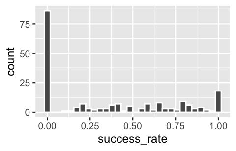

FIGURE 18.1: A histogram of the success rates for the 200 climbing expeditions.

18.1.1 Model building & simulation

Reflecting the grouped nature of our data, let \(Y_{ij}\) denote whether or not climber \(i\) in expedition \(j\) successfully summits their peak:

\[Y_{ij} = \begin{cases} 1 & \text{yes} \\ 0 & \text{no} \\ \end{cases}\]

There are several potential predictors of climber success in our dataset. We’ll consider only two: a climber’s age and whether they received supplemental oxygen in order to breathe more easily at high elevation. As such, define:

\[\begin{split} X_{ij1} & = \text{ age of climber $i$ in expedition $j$} \\ X_{ij2} & = \text{ whether or not climber $i$ in expedition $j$ received oxygen. } \\ \end{split}\]

By calculating the proportion of success at each age and oxygen use combination, we get a sense of how these factors are related to climber success (albeit a wobbly sense given the small sample sizes of some combinations). In short, it appears that climber success decreases with age and drastically increases with the use of oxygen:

# Calculate the success rate by age and oxygen use
data_by_age_oxygen <- climbers %>% 
  group_by(age, oxygen_used) %>% 
  summarize(success_rate = mean(success))

# Plot this relationship
ggplot(data_by_age_oxygen, aes(x = age, y = success_rate, 
                               color = oxygen_used)) + 
  geom_point()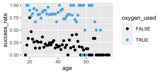

FIGURE 18.2: A scatterplot of the success rate among climbers by age and oxygen use.

In building a Bayesian model of this relationship, first recognize that the Bernoulli model is reasonable for our binary response variable \(Y_{ij}\). Letting \(\pi_{ij}\) be the probability that climber \(i\) in expedition \(j\) successfully summits their peak, i.e., that \(Y_{ij} = 1\),

\[Y_{ij} | \pi_{ij} \sim \text{Bern}(\pi_{ij}) .\]

Way back in Chapter 13, we explored a complete pooling approach to expanding this simple model into a logistic regression model of \(Y\) by a set of predictors \(X\):

\[\begin{split} Y_{ij}|\beta_0,\beta_1,\beta_2 & \stackrel{ind}{\sim} \text{Bern}(\pi_{ij}) \;\; \text{ with } \;\; \log\left(\frac{\pi_{ij}}{1 - \pi_{ij}}\right) = \beta_0 + \beta_1 X_{ij1} + \beta_2 X_{ij2} \\ \beta_{0c} & \sim N\left(m_0, s_0^2 \right) \\ \beta_1 & \sim N\left(m_1, s_1^2 \right) \\ \beta_2 & \sim N\left(m_2, s_2^2 \right). \\ \end{split}\]

This is a great start, BUT it doesn’t account for the grouping structure of our data. Instead, consider the following hierarchical alternative with independent, weakly informative priors tuned below by stan_glmer() and with a prior model for \(\beta_0\) expressed through the centered intercept \(\beta_{0c}\). After all, it makes more sense to think about the baseline success rate among the typical climber, \(\beta_{0c}\), than among 0-year-old climbers that don’t use oxygen, \(\beta_0\). To this end, we started our analysis with a weak understanding that the typical climber has a 0.5 probability of success, or a \(\text{log(odds of success)} = 0\).

\[\begin{equation} \begin{array}{rll} Y_{ij}|\beta_{0j},\beta_1, \beta_2 & \sim \text{Bern}(\pi_{ij}) & \text{(model within expedition $j$)}\\ \; \text{ with } & \log\left(\frac{\pi_{ij}}{1 - \pi_{ij}}\right) = \beta_{0j} + \beta_1 X_{ij1} + \beta_2 X_{ij2} & \\ \beta_{0j} | \beta_0, \sigma_0 & \stackrel{ind}{\sim} N(\beta_0, \sigma_0^2) & \text{(variability between expeditions)} \\ \beta_{0c} & \sim N\left(0, 2.5^2 \right) & \text{(global priors)}\\ \beta_1 & \sim N\left(0, 0.24^2 \right) & \\ \beta_2 & \sim N\left(0, 5.51^2 \right) & \\ \sigma_0 & \sim \text{Exp}(1). & \\ \end{array} \tag{18.1} \end{equation}\]

Equivalently, we can reframe this random intercepts logistic regression model by expressing the expedition-specific intercepts as tweaks to the global intercept,

\[\log\left(\frac{\pi_{ij}}{1 - \pi_{ij}}\right) = (\beta_0 + b_{0j}) + \beta_1 X_{ij1} + \beta_2 X_{ij2}\]

where \(b_{0j} | \sigma_0 \stackrel{ind}{\sim} N(0, \sigma_0^2)\). Consider the meaning of, and assumptions behind, the model parameters:

• The expedition-specific intercepts \(\beta_{0j}\) describe the underlying success rates, as measured by the log(odds of success), for each expedition \(j\). These acknowledge that some expeditions are inherently more successful than others.

• The expedition-specific intercepts \(\beta_{0j}\) are assumed to be Normally distributed around some global intercept \(\beta_0\) with standard deviation \(\sigma_0\). Thus, \(\beta_0\) describes the typical baseline success rate across all expeditions, and \(\sigma_0\) captures the between-group variability in success rates from expedition to expedition.

• \(\beta_1\) describes the global relationship between success and age when controlling for oxygen use. Similarly, \(\beta_2\) describes the global relationship between success and oxygen use when controlling for age.

Putting this all together, our random intercepts logistic regression model (18.1) makes the simplifying (but we think reasonable) assumption that expeditions might have unique intercepts \(\beta_{0j}\) but share common regression parameters \(\beta_1\) and \(\beta_2\). In plain language, though the underlying success rates might differ from expedition to expedition, being younger or using oxygen aren’t more beneficial in one expedition than in another.

To simulate the model posterior, the stan_glmer() code below combines the best of two worlds: family = binomial specifies that ours is a logistic regression model (à la Chapter 13) and the (1 | expedition_id) term in the model formula incorporates our hierarchical grouping structure (à la Chapter 17):

climb_model <- stan_glmer(
  success ~ age + oxygen_used + (1 | expedition_id), 
  data = climbers, family = binomial,
  prior_intercept = normal(0, 2.5, autoscale = TRUE),
  prior = normal(0, 2.5, autoscale = TRUE), 
  prior_covariance = decov(reg = 1, conc = 1, shape = 1, scale = 1),
  chains = 4, iter = 5000*2, seed = 84735
)

You’re encouraged to follow this simulation with a confirmation of the prior specifications and some MCMC diagnostics:

# Confirm prior specifications
prior_summary(climb_model)

# MCMC diagnostics
mcmc_trace(climb_model, size = 0.1)
mcmc_dens_overlay(climb_model)
mcmc_acf(climb_model)
neff_ratio(climb_model)
rhat(climb_model)

Whereas these diagnostics confirm that our MCMC simulation is on the right track, a posterior predictive check indicates that our model is on the right track. From each of 100 posterior simulated datasets, we record the proportion of climbers that were successful using the success_rate() function. These success rates range from roughly 37% to 41%, in a tight window around the actual observed 38.9% success rate in the climbers data.

# Define success rate function
success_rate <- function(x){mean(x == 1)}

# Posterior predictive check
pp_check(climb_model, nreps = 100,
         plotfun = "stat", stat = "success_rate") + 
  xlab("success rate")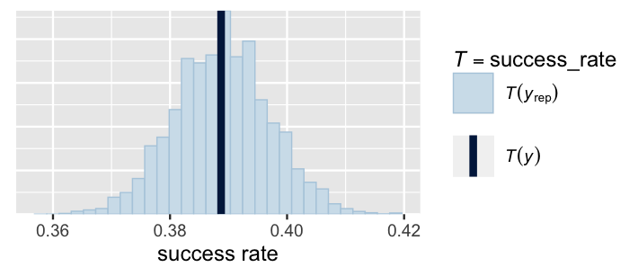

FIGURE 18.3: A posterior predictive check of the hierarchical logistic regression model of climbing success. The histogram displays the proportion of climbers that were successful in each of 100 posterior simulated datasets. The vertical line represents the observed proportion of climbers that were successful in the climbers data.

18.1.2 Posterior analysis

In our posterior analysis of mountain climber success, let’s focus on the global. Beyond being comforted by the fact that we’re correctly accounting for the grouping structure of our data, we aren’t interested in any particular expedition. With that, below are some posterior summaries for our global regression parameters \(\beta_0\), \(\beta_1\), and \(\beta_2\):

tidy(climb_model, effects = "fixed", conf.int = TRUE, conf.level = 0.80)
# A tibble: 3 x 5
  term            estimate std.error conf.low conf.high
  <chr>              <dbl>     <dbl>    <dbl>     <dbl>
1 (Intercept)      -1.42     0.479    -2.04     -0.822 
2 age              -0.0474   0.00910  -0.0594   -0.0358
3 oxygen_usedTRUE   5.79     0.478     5.20      6.43  

To begin, notice that the 80% posterior credible interval for age coefficient \(\beta_1\) is comfortably below 0. Thus, we have significant posterior evidence that, when controlling for whether or not a climber uses oxygen, the likelihood of success decreases with age. More specifically, translating the information in \(\beta_1\) from the log(odds) to the odds scale, there’s an 80% chance that the odds of successfully summiting drop somewhere between 3.5% and 5.8% for every extra year in age: \((e^{-0.0594}, e^{-0.0358}) = (0.942, 0.965)\). Similarly, the 80% posterior credible interval for the oxygen_usedTRUE coefficient \(\beta_2\) provides significant posterior evidence that, when controlling for age, the use of oxygen dramatically increases a climber’s likelihood of summiting the peak. There’s an 80% chance that the use of oxygen could correspond to anywhere between a 182-fold increase to a 617-fold increase in the odds of success: \((e^{5.2}, e^{6.43}) = (182, 617)\). Oxygen please!

Combining our observations on \(\beta_1\) and \(\beta_2\), the posterior median model of the relationship between climbers’ log(odds of success) and their age (\(X_1\)) and oxygen use (\(X_2\)) is

\[\text{log}\left(\frac{\pi}{1 - \pi}\right) = -1.42 - 0.0474 X_1 + 5.79 X_2.\]

Or, on the probability of success scale:

\[\pi = \frac{e^{-1.42 - 0.0474 X_1 + 5.79 X_2}}{1 + e^{-1.42 - 0.0474 X_1 + 5.79 X_2}}.\]

This posterior median model merely represents the center among a range of posterior plausible relationships between success, age, and oxygen use. To get a sense for this range, Figure 18.4 plots 100 posterior plausible alternative models. Both with oxygen and without, the probability of success decreases with age. Further, at any given age, the probability of success is drastically higher when climbers use oxygen. However, our posterior certainty in these trends varies quite a bit by age. We have much less certainty about the success rate for older climbers on oxygen than for younger climbers on oxygen, for whom the success rate is uniformly high. Similarly, but less drastically, we have less certainty about the success rate for younger climbers who don’t use oxygen than for older climbers who don’t use oxygen, for whom the success rate is uniformly low.

climbers %>%
  add_fitted_draws(climb_model, n = 100, re_formula = NA) %>%
  ggplot(aes(x = age, y = success, color = oxygen_used)) +
    geom_line(aes(y = .value, group = paste(oxygen_used, .draw)), 
              alpha = 0.1) + 
    labs(y = "probability of success")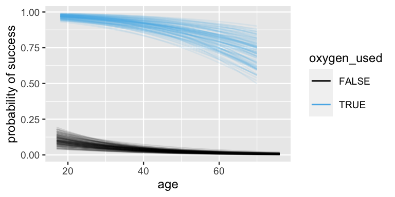

FIGURE 18.4: 100 posterior plausible models for the probability of climbing success by age and oxygen use.

18.1.3 Posterior classification

Suppose four climbers set out on a new expedition. Two are 20 years old and two are 60 years old. Among both age pairs, one climber plans to use oxygen and the other does not:

# New expedition
new_expedition <- data.frame(
  age = c(20, 20, 60, 60), oxygen_used = c(FALSE, TRUE, FALSE, TRUE), 
  expedition_id = rep("new", 4))
new_expedition
  age oxygen_used expedition_id
1  20       FALSE           new
2  20        TRUE           new
3  60       FALSE           new
4  60        TRUE           new

Naturally, they each want to know the probability that they’ll reach their summit. For a reminder on how to simulate a posterior predictive model for a new group from scratch, please review Section 16.5. Here we jump straight to the posterior_predict() shortcut function to simulate 20,000 0-or-1 posterior predictions for each of our 4 new climbers:

# Posterior predictions of binary outcome
set.seed(84735)
binary_prediction <- posterior_predict(climb_model, newdata = new_expedition)

# First 3 prediction sets
head(binary_prediction, 3)
     1 2 3 4
[1,] 0 1 0 1
[2,] 0 1 0 1
[3,] 0 1 0 1

For each climber, the probability of success is approximated by the observed proportion of success among their 20,000 posterior predictions. Since these probabilities incorporate uncertainty in the baseline success rate of the new expedition, they are more moderate than the global trends observed in Figure 18.4:

# Summarize the posterior predictions of Y
colMeans(binary_prediction)
     1      2      3      4 
0.2788 0.8040 0.1440 0.6515 

These posterior predictions provide more insight into the connections between age, oxygen, and success. For example, our posterior prediction is that climber 1, who is 20 years old and does not plan to use oxygen, has a 27.88% chance of summiting the peak. This probability is naturally lower than for climber 2, who is also 20 but does plan to use oxygen. It’s also higher than the posterior prediction of success for climber 3, who also doesn’t plan to use oxygen but is 60 years old. Overall, the posterior prediction of success is highest for climber 2, who is younger and plans to use oxygen, and lowest for climber 3, who is older and doesn’t plan to use oxygen.

In Chapter 13 we discussed the option of turning such posterior probability predictions into posterior classifications of binary outcomes: yes or no, do we anticipate that the climber will succeed or not? If we used a simple 0.5 posterior probability cut-off to make this determination, we would recommend that climbers 1 and 3 not join the expedition (at least, not without oxygen) and give climbers 2 and 4 the go ahead. Yet in this particular context, we should probably leave it up to individual climbers to interpret their own results and make their own yes-or-no decisions about whether to continue on their expedition. For example, a 65.16% chance of success might be worth the hassle and risk to some but not to others.

18.1.4 Model evaluation

To conclude our climbing analysis, let’s ask: Is our hierarchical logistic model a good model? Long story short, the answer is yes. First, our model is fair. The data we used are part of public record and we do not foresee our analysis having any negative impact on individuals or society. (Again, boring answers to the question of fairness are the best kind.) Second, our posterior predictive check in Figure 18.3 demonstrated that our model doesn’t seem too wrong – our posterior simulated success rates hover around the observed success rate in our data. Finally, to the question of posterior classification accuracy, we can compare our posterior classifications of success to the actual outcomes for the 2076 climbers in our dataset. By default, let’s start out with a probability cut-off of 0.5 – if a climber’s probability of success exceeds 0.5, we’ll predict that they’ll succeed. We implement and evaluate this classification rule using classification_summary() below.

set.seed(84735)
classification_summary(data = climbers, model = climb_model, cutoff = 0.5)

$confusion_matrix
     y    0   1
 FALSE 1174  95
  TRUE   77 730

$accuracy_rates
                       
sensitivity      0.9046
specificity      0.9251
overall_accuracy 0.9171

Overall, under this classification rule, our model successfully predicts the outcomes for 91.71% of our climbers. This is pretty fantastic given that we’re only utilizing information on the climbers’ ages and oxygen use, among many possible other considerations (e.g., destination, season, etc.). Yet given the consequences of misclassification in this particular context (e.g., risk of injury), we should prioritize specificity, our ability to anticipate when a climber might not succeed. To this end, our model correctly predicted only 92.51% of the climbing failures. To increase this rate, we can change the probability cut-off in our classification rule.

What cut-off can we utilize to achieve a specificity of at least 95% while also maintaining the highest possible sensitivity?

In general, to increase specificity, we can increase the probability cut-off, thereby making it more difficult to predict “success.” After some trial and error, it seems that cut-offs of roughly 0.65 or higher will achieve a desired 95% specificity level. This switch to 0.65 naturally decreases the sensitivity of our posterior classifications, from 90.46% to 81.54%, and thus our ability to detect when a climber will be successful. We think the added caution is worth it.

set.seed(84735)
classification_summary(data = climbers, model = climb_model, cutoff = 0.65)

$confusion_matrix
     y    0   1
 FALSE 1214  55
  TRUE  149 658

$accuracy_rates
                       
sensitivity      0.8154
specificity      0.9567
overall_accuracy 0.9017

18.2 Hierarchical Poisson & Negative Binomial regression

Vacation rental services, such as AirBnB, offer travelers alternatives to hotel rooms. The AirBnB inventory and price range are wide, leading us to ask: why do some listings have more reviews (hence presumably more guests) than others? Beyond a vague baseline understanding that the typical listing has around 20 reviews, we’re unsure of the dynamics in the AirBnB market, and thus will otherwise utilize weakly informative priors. We’ll balance these priors by the airbnb data in the bayesrules package, originally collated by Trinh and Ameri (2016) and distributed by Legler and Roback (2021). This dataset contains information on 1561 listings across 43 Chicago neighborhoods, and hence multiple listings per neighborhood:

# Load data
data(airbnb)

# Number of listings
nrow(airbnb)
[1] 1561

# Number of neighborhoods
airbnb %>% 
  summarize(nlevels(neighborhood))
  nlevels(neighborhood)
1                    43

We’re not interested in these neighborhoods in particular. Rather, we’d like to use these data on these neighborhoods to learn about the broader AirBnB market. However, since listings within the same neighborhood share many features (e.g., similar location, amenities, public transit), it would be a mistake to assume their independence. Thus, to reflect and study the variability in the number of AirBnB reviews between and within neighborhoods, we’ll incorporate the neighborhood grouping structure in our analysis.

18.2.1 Model building & simulation

In exploring why the number of reviews varies from AirBnB listing to listing, we’ll consider two possible factors: its overall user rating (on a 1 to 5 scale) and the privacy allotted by its room_type, i.e., whether the renter gets an entire private unit, gets a private room within a shared unit, or shares a room. More specifically, for listing \(i\) in neighborhood \(j\), we will model response variable

\[Y_{ij} = \text{ number of reviews }\]

by visitor rating \(X_{ij1}\) and room type, where an entire private unit is the reference level and we have indicator variables for the two other room types:

\[X_{ij2} = \begin{cases} 1 & \text{private room} \\ 0 & \text{otherwise} \\ \end{cases} \;\; \text{ and } \;\; X_{ij3} = \begin{cases} 1 & \text{shared room} \\ 0 & \text{otherwise} \\ \end{cases}\]

Figure 18.5 displays the trends in the number of reviews as well as their relationship with a listing’s rating and room type. In examining the variability in \(Y_{ij}\) alone, note that the majority of listings have fewer than 20 reviews, though there’s a long right skew. Further, the volume of reviews tends to increase with ratings and privacy levels.

ggplot(airbnb, aes(x = reviews)) + 
  geom_histogram(color = "white", breaks = seq(0, 200, by = 10))
ggplot(airbnb, aes(y = reviews, x = rating)) + 
  geom_jitter()
ggplot(airbnb, aes(y = reviews, x = room_type)) + 
  geom_violin()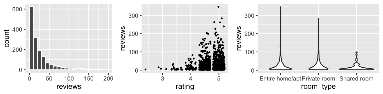

FIGURE 18.5: Plots of the number of reviews received across AirBnB listings (left) as well as the relationship of the number of reviews with a listing’s rating (middle) and room type (right).

We can further break down these dynamics within each neighborhood. We show just three here to conserve precious space: Albany Park (a residential neighborhood in northern Chicago), East Garfield Park (a residential neighborhood in central Chicago), and The Loop (a commercial district and tourist destination). In general, notice that Albany Park listings tend to have fewer reviews, no matter their rating or room type.

airbnb %>% 
  filter(neighborhood %in% 
           c("Albany Park", "East Garfield Park", "The Loop")) %>% 
  ggplot(aes(y = reviews, x = rating, color = room_type)) + 
    geom_jitter() + 
    facet_wrap(~ neighborhood)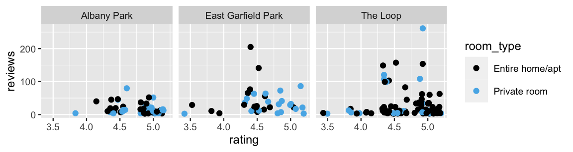

FIGURE 18.6: A scatterplot of an AirBnB listing’s number of reviews by its rating and room type, for three neighborhoods.

In building a regression model for the number of reviews, the first step is to consider reasonable probability models for data \(Y_{ij}\). Since the \(Y_{ij}\) values are non-negative skewed counts, a Poisson model is a good starting point. Specifically, letting rate \(\lambda_{ij}\) denote the expected number of reviews received by listing \(i\) in neighborhood \(j\),

\[Y_{ij} | \lambda_{ij} \sim \text{Pois}(\lambda_{ij}) .\]

The hierarchical Poisson regression model below builds this out to incorporate (1) the rating and room type predictors (\(X_{ij1}\), \(X_{ij2}\), \(X_{ij3}\)) and (2) the airbnb data’s grouped structure. Beyond a general understanding that the typical listing has around 20 reviews (hence \(\log(20) \approx 3\) logged reviews), this model utilizes independent, weakly informative priors tuned by stan_glmer():

\[\begin{equation} \begin{array}{rl} Y_{ij}|\beta_{0j},\beta_1, \beta_2, \beta_3 & \sim \text{Pois}(\lambda_{ij}) \;\; \text{ with } \;\; \log(\lambda_{ij}) = \beta_{0j} + \beta_1 X_{ij1} + \beta_2 X_{ij2} + \beta_3 X_{ij3} \\ \beta_{0j} | \beta_0, \sigma_0 & \stackrel{ind}{\sim} N(\beta_0, \sigma_0^2)\\ \beta_{0c} & \sim N\left(3, 2.5^2 \right)\\ \beta_{1} & \sim N\left(0, 7.37^2 \right)\\ \beta_{2} & \sim N\left(0, 5.04^2 \right)\\ \beta_{3} & \sim N\left(0, 14.19^2 \right)\\ \sigma_0 & \sim \text{Exp}(1). \\ \end{array} \tag{18.2} \end{equation}\]

Taking a closer look, this model assumes that neighborhoods might have unique intercepts \(\beta_{0j}\) but share common regression parameters \((\beta_1, \beta_2, \beta_3)\). In plain language: though some neighborhoods might be more popular AirBnB destinations than others (hence their listings tend to have more reviews), the relationship of reviews with rating and room type is the same for each neighborhood. For instance, ratings aren’t more influential to reviews in one neighborhood than in another. This assumption greatly simplifies our analysis while still accounting for the grouping structure in the data. To simulate the posterior, we specify our family = poisson data structure and incorporate the neighborhood-level grouping structure through (1 | neighborhood):

airbnb_model_1 <- stan_glmer(
  reviews ~ rating + room_type + (1 | neighborhood), 
  data = airbnb, family = poisson,
  prior_intercept = normal(3, 2.5, autoscale = TRUE),
  prior = normal(0, 2.5, autoscale = TRUE), 
  prior_covariance = decov(reg = 1, conc = 1, shape = 1, scale = 1),
  chains = 4, iter = 5000*2, seed = 84735
)

Before getting too excited, let’s do a quick pp_check():

pp_check(airbnb_model_1) + 
  xlim(0, 200) + 
  xlab("reviews")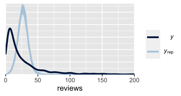

FIGURE 18.7: A posterior predictive check of the AirBnB Poisson regression model.

Figure 18.7 indicates that our hierarchical Poisson regression model significantly underestimates the variability in reviews from listing to listing, while overestimating the typical number of reviews. We’ve been here before! Recall from Chapter 12 that an underlying Poisson regression assumption is that, at any set of predictor values, the average number of reviews is equal to the variance in reviews:

\[E(Y_{ij}) = \text{Var}(Y_{ij}) = \lambda_{ij} .\]

The pp_check() calls this assumption into question. To address the apparent overdispersion in the \(Y_{ij}\) values, we swap out the Poisson model in (18.2) for the more flexible Negative Binomial model, picking up the additional reciprocal dispersion parameter \(r > 0\):

\[\begin{equation} \begin{array}{rl} Y_{ij}|\beta_{0j},\beta_1, \beta_2, \beta_3, r & \sim \text{NegBin}(\mu_{ij}, r) \;\; \text{ with } \;\; \log(\mu_{ij}) = \beta_{0j} + \beta_1 X_{ij1} + \beta_2 X_{ij2} + \beta_3 X_{ij3} \\ \beta_{0j} | \beta_0, \sigma_0 & \stackrel{ind}{\sim} N(\beta_0, \sigma_0^2) \\ \beta_{0c} & \sim N\left(3, 2.5^2 \right) \\ \beta_1 & \sim N\left(0, 7.37^2 \right) \\ \beta_2 & \sim N\left(0, 5.04^2 \right) \\ \beta_3 & \sim N\left(0, 14.19^2 \right) \\ r & \sim \text{Exp}(1) \\ \sigma_0 & \sim \text{Exp}(1) \\ \end{array} \tag{18.3} \end{equation}\]

Equivalently, we can express the random intercepts as tweaks to the global intercept,

\[\log(\mu_{ij}) = (\beta_0 + b_{0j}) + \beta_1 X_{ij1} + \beta_2 X_{ij2} + \beta_3 X_{ij3}\]

where \(b_{0j} | \sigma_0 \stackrel{ind}{\sim} N(0, \sigma_0^2)\). To simulate the posterior of the hierarchical Negative Binomial regression model, we can swap out family = poisson for family = neg_binomial_2:

airbnb_model_2 <- stan_glmer(
  reviews ~ rating + room_type + (1 | neighborhood), 
  data = airbnb, family = neg_binomial_2,
  prior_intercept = normal(3, 2.5, autoscale = TRUE),
  prior = normal(0, 2.5, autoscale = TRUE), 
  prior_aux = exponential(1, autoscale = TRUE),
  prior_covariance = decov(reg = 1, conc = 1, shape = 1, scale = 1),
  chains = 4, iter = 5000*2, seed = 84735
)

Though not perfect, the Negative Binomial model does a much better job of capturing the behavior in reviews from listing to listing:

pp_check(airbnb_model_2) + 
  xlim(0, 200) + 
  xlab("reviews")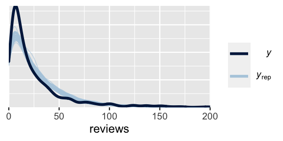

FIGURE 18.8: A posterior predictive check of the Negative Binomial regression model of AirBnB reviews.

18.2.2 Posterior analysis

Let’s now make meaning of our posterior simulation results, beginning with the global relationship of reviews with ratings and room type, \(\log(\lambda_{ij}) = \beta_0 + \beta_1 X_{ij1} + \beta_2 X_{ij2} + \beta_3 X_{ij3}\), or:

\[\lambda_{ij} = e^{\beta_0 + \beta_1 X_{ij1} + \beta_2 X_{ij2} + \beta_3 X_{ij3}}.\]

Below are posterior summaries of our global parameters \((\beta_0,\beta_1, \beta_2, \beta_3)\). The posterior model of \(\beta_1\) reflects a significant and substantive positive association between reviews and rating. When controlling for room type, there’s an 80% chance that the volume of reviews increases somewhere between 1.17 and 1.45 times, or 17 and 45 percent, for every extra point in rating: (\(e^{0.154}\), \(e^{0.371}) = (1.17, 1.45)\). In contrast, the posterior model of \(\beta_3\) illustrates that shared rooms are negatively associated with reviews. When controlling for ratings, there’s an 80% chance that the volume of reviews for shared room listings is somewhere between 52 and 76 percent as high as for listings that are entirely private: \((e^{-0.659}, e^{-0.275}) = (0.52, 0.76)\).

tidy(airbnb_model_2, effects = "fixed", conf.int = TRUE, conf.level = 0.80)
# A tibble: 4 x 5
  term            estimate std.error conf.low conf.high
  <chr>              <dbl>     <dbl>    <dbl>     <dbl>
1 (Intercept)       1.99      0.405   1.48e+0     2.52 
2 rating            0.265     0.0852  1.54e-1     0.371
3 room_typePriva…   0.0681    0.0520  9.54e-4     0.136
4 room_typeShare…  -0.471     0.149  -6.59e-1    -0.275

Let’s also peak at some neighborhood-specific AirBnB models,

\[\lambda_{ij} = e^{\beta_{0j} + \beta_1 X_{ij1} + \beta_2 X_{ij2} + \beta_3 X_{ij3}}\]

where \(\beta_{0j}\), the baseline review rate, varies from neighborhood to neighborhood. We’ll again focus on just three neighborhoods: Albany Park, East Garfield Park, and The Loop. The below posterior summaries evaluate the differences between these neighborhoods’ baselines and the global intercept, \(b_{0j} = \beta_{0j} - \beta_0\):

tidy(airbnb_model_2, effects = "ran_vals", 
     conf.int = TRUE, conf.level = 0.80) %>% 
  select(level, estimate, conf.low, conf.high) %>% 
  filter(level %in% c("Albany_Park", "East_Garfield_Park", "The_Loop"))
# A tibble: 3 x 4
  level              estimate conf.low conf.high
  <chr>                 <dbl>    <dbl>     <dbl>
1 Albany_Park         -0.234   -0.427    -0.0548
2 East_Garfield_Park   0.205    0.0385    0.397 
3 The_Loop             0.0101  -0.0993    0.124 

Note that AirBnB listings in Albany Park have atypically few reviews, those in East Garfield Park have atypically large numbers of reviews, and those in The Loop do not significantly differ from the average. Though not dramatic, these differences from neighborhood to neighborhood play out in posterior predictions. For example, below we simulate posterior predictive models of the number of reviews for three listings that each have a 5 rating and each offer privacy, yet they’re in three different neighborhoods. Given the differing review baselines in these neighborhoods, we anticipate that the Albany Park listing will have fewer reviews than the East Garfield Park listing, though the predictive ranges are quite wide:

# Posterior predictions of reviews
set.seed(84735)
predicted_reviews <- posterior_predict(
  airbnb_model_2, 
  newdata = data.frame(
    rating = rep(5, 3), 
    room_type = rep("Entire home/apt", 3), 
    neighborhood = c("Albany Park", "East Garfield Park", "The Loop")))
mcmc_areas(predicted_reviews, prob = 0.8) +
  ggplot2::scale_y_discrete(
    labels = c("Albany Park", "East Garfield Park", "The Loop")) + 
  xlim(0, 150) + 
  xlab("reviews")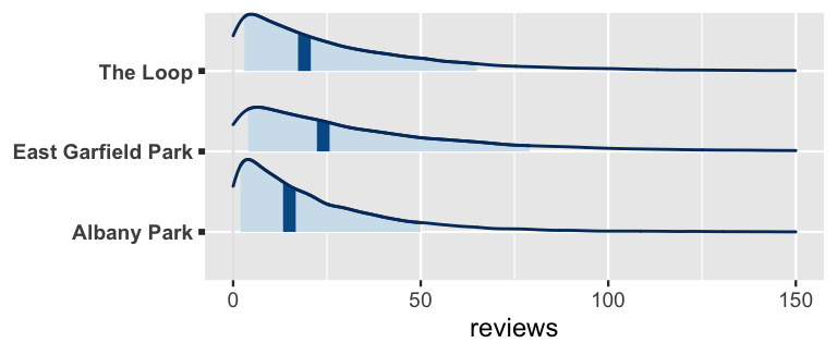

FIGURE 18.9: Posterior predictive models for the number of reviews for AirBnB listings in three different neighborhoods.

18.2.3 Model evaluation

To wrap things up, let’s formally evaluate the quality of our listing analysis. First, to the question of whether or not our model is fair. Kinda. In answering our research question about AirBnB, we tried to learn something from the data available to us. What was available was information about the AirBnB market in Chicago. Thus, we’d be hesitant to use our analysis for anything more than general conclusions about the broader market. Second, our posterior predictive check in Figure 18.8 indicated that our model isn’t TOO wrong – at least it’s much better than taking a Poisson approach! Finally, our posterior predictions of review counts are not very accurate. The observed number of reviews for a listing tends to be 18 reviews, or 0.68 standard deviations, from its posterior mean prediction. This level of error is quite large on the scale of our data – though the number of reviews per listing ranges from roughly 0 to 200, most listings have below 20 reviews (Figure 18.5). To improve our prediction of the number of reviews a listing receives, we might incorporate additional predictors into our analysis.

set.seed(84735)
prediction_summary(model = airbnb_model_2, data = airbnb)
   mae mae_scaled within_50 within_95
1 17.7      0.678    0.5183    0.9571

18.3 Chapter summary

In Chapter 18 we combined the Unit 3 principles of generalized linear models with the Unit 4 principles of hierarchical modeling, thereby expanding our hierarchical toolkit to include Normal, Poisson, Negative Binomial, and logistic regression. In general, let \(E(Y_{ij}|\ldots)\) denote the expected value of \(Y_{ij}\) as defined by its model structure. For all hierarchical generalized linear models, the dependence of \(E(Y_{ij}|\ldots)\) on a linear combination of \(p\) predictors \((X_{ij1}, X_{ij2}, ..., X_{ijp})\) is expressed by

\[\begin{split} g\left(E(Y_{ij}|\ldots)\right) & = \beta_{0j} + \beta_{1j} X_{ij1} + \beta_{2j} X_{ij2} + \cdots + \beta_{pj} X_{ijp} \\ & = (\beta_0 + b_{0j}) + (\beta_1 + b_{1j}) X_{ij1} + (\beta_2 + b_{2j}) X_{ij2} + \cdots + (\beta_p + b_{pj}) X_{ijp} \\ \end{split}\]

where (1) any group-specific parameter \(\beta_{kj}\) can be replaced by a global parameter \(\beta_k\) in cases of little variability in the \(\beta_{kj}\) between groups and (2) the link function \(g(\cdot)\) depends upon the model structure:

model	link function
\(Y_{ij} | \ldots \sim N(\mu_{ij}, \sigma_y^2)\)	\(g(\mu_{ij}) = \mu_{ij}\)
\(Y_{ij} | \ldots \sim \text{Pois}(\lambda_{ij})\)	\(g(\lambda_{ij})= \log(\lambda_{ij})\)
\(Y_{ij} | \ldots \sim \text{NegBinom}(\mu_{ij}, r)\)	\(g(\mu_{ij})= \log(\mu_{ij})\)
\(Y_{ij} | \ldots \sim \text{Bern}(\pi_{ij})\)	\(g(\pi_{ij}) = \log\left(\frac{\pi_{ij}}{1 - \pi_{ij}}\right)\)

18.4 Exercises

18.4.1 Applied & conceptual exercises

Exercise 18.1 (We know how to do a lot of stuff) For each model scenario, specify an appropriate structure for the data model, note whether the model is hierarchical, and if so, identify the grouping variable. Though you do not need to simulate the models, be sure to justify your selections using the data provided. To learn more about these datasets, type ?name_of_dataset into the console.

1. Using the coffee_ratings data in R, researchers wish to model whether a batch of coffee beans is of the Robusta species based on its flavor.
2. Using the trees data in R, researchers wish to model a tree’s Height by its Girth.
3. Using the radon data in the rstanarm package, researchers wish to model a home’s log_radon levels by its log_uranium levels.
4. Using the roaches data in the rstanarm package, researchers wish to model the number of roaches in an urban apartment by whether or not the apartment has received a pest control treatment.

Exercise 18.2 (Book banning: setting up the model) People have both failed and succeeded at getting books banned, and hence ideas censored, from public libraries and education. In the following exercises, you’ll explore whether certain book characteristics can help predict whether or not a book challenge is successful. To do so, you’ll balance weakly informative priors with the book_banning data in the bayesrules package. This data, collected by Fast and Hegland (2011) and presented by Legler and Roback (2021), includes features and outcomes for 931 book challenges made in the US between 2000 and 2010. Let \(Y_{ij}\) denote the outcome of the \(i\)th book challenge in state \(j\), i.e., whether or not the book was removed. You’ll consider three potential predictors of outcome: whether the reasons for the challenge include concern about violent material (\(X_{ij1}\)), antifamily material (\(X_{ij2}\)), or the use of inappropriate language (\(X_{ij3}\)).

1. In your book banning analysis, you’ll use the state in which the book challenge was made as a grouping variable. Explain why it’s reasonable (and important) to assume that the book banning outcomes within any given state are dependent.
2. Write out an appropriate hierarchical regression model of \(Y_{ij}\) by \((X_{ij1},X_{ij2},X_{ij3})\) using formal notation. Assume each state has its own intercept, but that the states share the same predictor coefficients.
3. Dig into the book_banning data. What state had the most book challenges? The least?
4. Which state has the greatest book removal rate? The smallest?
5. Visualize and discuss the relationships between the book challenge outcome and the three predictors.

Exercise 18.3 (Book banning: simulating the model) Next, let’s simulate and dig into the posterior model of the book banning parameters.

1. Simulate the posterior of your hierarchical book banning model. Construct trace, density, and autocorrelation plots of the chain output.
2. Report the posterior median global model. Interpret each number in this model.
3. Are each of violence, anti-family material, and inappropriate language significantly linked to the outcome of a book challenge (when controlling for the others)? Explain.
4. What combination of book features is most commonly associated with a book that’s banned? With a book that’s not banned? Explain.

Exercise 18.4 (Book banning: will the book be banned?)

1. How accurate are your model’s posterior predictions of whether a book will be banned? Provide evidence.
2. Interpret the posterior medians of \(b_{0j} = \beta_{0j} - \beta_0\) for two states \(j\): Kansas (KS) and Oregon (OR).
3. Suppose a book is challenged in both Kansas and Oregon for its language, but not for violence or anti-family material. Construct and compare posterior models for whether or not the book will be banned in these two states.

Exercise 18.5 (Basketball!) The Women’s National Basketball Association (WNBA) is a professional basketball league in North America. Founded in the mid-1990s, the league has grown to include twelve teams. Though teams might have up to 12 players, only five play at a time. Players then rotate in and out throughout the game, with the best combination of players typically starting the game. The goal of our analysis is to better understand why some players get more game time than other players. Beyond the general understanding that the typical player gets 400 minutes of game time throughout the season, we’ll balance weakly informative priors with the basketball data in the bayesrules package. This data includes information about various players from the 2019 season including:

variable	meaning
total_minutes	the total number of minutes played throughout the season
games_played	the number of games played throughout the season
starter	whether or not the player started in more than half of the
	games that they played
avg_points	the average number of points scored per game
team	team name

1. How many players are in the dataset?
2. How many teams are represented in the dataset?
3. Construct and discuss a plot of total_minutes vs avg_points and starter. Is this what you would expect to see?
4. Construct and discuss a plot of total_minutes vs games_played and starter. NOTE: Incorporating games_played into our analysis provides an important point of comparison for the total number of minutes played.

Exercise 18.6 (Basketball! Build a model)

1. Using formal notation, write out a hierarchical Poisson regression model of total_minutes by avg_points, starter, and games_played. Use team as the grouping variable.
2. Explain why the Poisson might be a reasonable model structure here, and why it might not be.
3. Explain why it’s important to include team as a grouping variable.
4. Simulate this model using weakly informative priors and perform a pp_check().

Exercise 18.7 (Basketball! Normal or Poisson or Negative Binomial?) Above, you analyzed a player’s total number of minutes played using a Poisson hierarchical regression model. Redo this analysis using a Normal and a Negative Binomial hierarchical model. Evaluate and compare the three models, and explain which you prefer.

Exercise 18.8 (More basketball!) Utilize your final chosen model (Poisson, Normal, or Negative Binomial) to explore the relationship between the total number of minutes played by a player and their average points per game in more depth.

1. Summarize your key findings. Some things to consider along the way: Can you interpret every model parameter (both global and team-specific)? Can you summarize the key trends? Which trends are significant? How good is your model?

2. Predict the total number of minutes that a player will get throughout a season if they play in 30 games, they start each game, and they score an average of 15 points per game.

18.4.2 Open-ended exercises

Exercise 18.9 (Open exercise: basketball analysis with multiple predictors) In this open-ended exercise, complete an analysis of the number of games started by WNBA players using multiple predictors of your choosing.

Exercise 18.10 (Open exercise: more climbing) In Chapter 18, you analyzed the relationship of a climber’s success with their age and oxygen use. In this open-ended exercise, continue your climbing analysis by considering other possible predictors. These might include any combination of personal attributes (age, oxygen_used, injured), time attributes (year, season), or attributes of the climb itself (highpoint_metres, height_metres).

References

Fast, Shannon, and Thomas Hegland. 2011. “Book Challenges: A Statistical Examination.” Project for Statistics 316-Advanced Statistical Modeling, St. Olaf College.

Legler, Julie, and Paul Roback. 2021. Beyond Multiple Linear Regression: Applied Generalized Linear Models and Multilevel Models in R. Chapman; Hall/CRC. https://bookdown.org/roback/bookdown-BeyondMLR/.

———. 2020b. “Himalayan Climbing Expeditions.” TidyTuesday Github Repostitory. https://github.com/rfordatascience/tidytuesday/tree/master/data/2020/2020-09-22.

The Himalayan Database. 2020. https://www.himalayandatabase.com/.

Trinh, Ly, and Pony Ameri. 2016. “AirBnB Price Determinants: A Multilevel Modeling Approach.” Project for Statistics 316-Advanced Statistical Modeling, St. Olaf College.

---

76. For example, the observed season categories (Autumn, Spring, Summer, Winter) are a fixed and complete set of options, not a random sample of categories from a broader population of seasons.↩︎