Chapter 5 Conjugate Families

In the novel Anna Karenina, Tolstoy wrote “Happy families are all alike; every unhappy family is unhappy in its own way.” In this chapter we will learn about conjugate families, which are all alike in the sense that they make the authors very happy. Read on to learn why.

• Practice building Bayesian models. You will build Bayesian models by practicing how to recognize kernels and make use of proportionality.
• Familiarize yourself with conjugacy. You will learn about what makes a prior conjugate and why this is a helpful property. In brief, conjugate priors make it easier to build posterior models. Conjugate priors spark joy!

Getting started

To prepare for this chapter, note that we’ll be using some new Greek letters throughout our analysis: λ$\lambda$ = lambda, μ$\mu$ = mu or “mew,” σ$\sigma$ = sigma, τ$\tau$ = tau, and θ$\theta$ = theta. Further, load the packages below.

library(bayesrules)
library(tidyverse)

5.1 Revisiting choice of prior

How do we choose a prior? In Chapters 3 and 4 we used the flexibility of the Beta model to reflect our prior understanding of a proportion parameter π∈[0,1]$\pi \in [0,1]$. There are other criteria to consider when choosing a prior model:

• Computational ease
  Especially if we don’t have access to computing power, it is helpful if the posterior model is easy to build.
• Interpretability
  We’ve seen that posterior models are a compromise between the data and the prior model. A posterior model is interpretable, and thus more useful, when you can look at its formulation and identify the contribution of the data relative to that of the prior.

The Beta-Binomial has both of these criteria covered. Its calculation is easy. Once we know the Beta(α,β$\alpha ,\beta$) prior hyperparameters and the observed data Y=y$Y=y$ for the Bin(n,π$n,\pi$) model, the Beta(α+y,β+n−y$\alpha +y,\beta +n-y$) posterior model follows. This posterior reflects the influence of the data, through the values of y$y$ and n$n$, relative to the prior hyperparameters α$\alpha$ and β$\beta$. If α$\alpha$ and β$\beta$ are large relative to the sample size n$n$, then the posterior will not budge that much from the prior. However, if the sample size n$n$ is large relative to α$\alpha$ and β$\beta$, then the data will take over and be more influential in the posterior model. In fact, the Beta-Binomial belongs to a larger class of prior-data combinations called conjugate families that enjoy both computational ease and interpretable posteriors. Recall a general definition similar to that from Chapter 3.

Conjugate prior

Let the prior model for parameter θ$\theta$ have pdf f(θ)$f\left(\theta \right)$ and the model of data Y$Y$ conditioned on θ$\theta$ have likelihood function L(θ|y)$L\left(\theta |y\right)$. If the resulting posterior model with pdf f(θ|y)∝f(θ)L(θ|y)$f\left(\theta |y\right)\propto f\left(\theta \right)L\left(\theta |y\right)$ is of the same model family as the prior, then we say this is a conjugate prior.

To emphasize the utility (and fun!) of conjugate priors, it can be helpful to consider a non-conjugate prior. Let parameter π$\pi$ be a proportion between 0 and 1 and suppose we plan to collect data Y$Y$ where, conditional on π$\pi$, Y|π∼Bin(n,π)$Y|\pi \sim \text{Bin}(n,\pi )$. Instead of our conjugate Beta(α,β)$\text{Beta}(\alpha ,\beta )$ prior for π$\pi$, let’s try out a non-conjugate prior with pdf f(π)$f\left(\pi \right)$, plotted in Figure 5.1:

f(π)=e−eπ for π∈[0,1].$$\begin{array}{}f\left(\pi \right)=e-e^{\pi }\text{for}\pi \in [0,1].& \text{(5.1)}\end{array}$$

Though not a Beta pdf, f(π)$f\left(\pi \right)$ is indeed a valid pdf since f(π)$f\left(\pi \right)$ is non-negative on the support of π$\pi$ and the area under the pdf is 1, i.e., ∫10f(π)=1${\int }_0^{1}f\left(\pi \right)=1$.

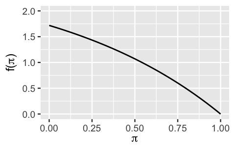
FIGURE 5.1: A non-conjugate prior for π$\pi$.

Next, suppose we observe Y=10$Y=10$ successes from n=50$n=50$ independent trials, all having the same probability of success π$\pi$. The resulting Binomial likelihood function of π$\pi$ is:

L(π|y=10)=(5010)π10(1−π)40 for π∈[0,1].$$L(\pi |y=10)=\left(\begin{array}{c}50\\ 10\end{array}\right){\pi }^{10}(1-\pi {)}^{40}\text{for}\pi \in [0,1].$$

Recall from Chapter 3 that, when we put the prior and the likelihood together, we are already on our path to finding the posterior model with pdf

f(π|y=10)∝f(π)L(π|y=10)=(e−eπ)⋅(5010)π10(1−π)40.$$f(\pi |y=10)\propto f\left(\pi \right)L(\pi |y=10)=(e-e^{\pi })\cdot (\frac{50}{10}){\pi }^{10}(1-\pi {)}^{40}.$$

As we did in Chapter 3, we will drop all constants that do not depend on π$\pi$ since we are only specifying f(π|y)$f\left(\pi |y\right)$ up to a proportionality constant:

f(π|y)∝(e−eπ)π10(1−π)40.$$f\left(\pi |y\right)\propto (e-e^{\pi }){\pi }^{10}(1-\pi {)}^{40}.$$

Notice here that our non-Beta prior didn’t produce a neat and clean answer for the exact posterior model (fully specified and not up to a proportionality constant). We cannot squeeze this posterior pdf kernel into a Beta box or any other familiar model for that matter. That is, we cannot rewrite (e−eπ)π10(1−π)40$(e-e^{\pi }){\pi }^{10}(1-\pi {)}^{40}$ so that it shares the same structure as a Beta kernel, π◼−1(1−π)◼−1${\pi }^{■-1}(1-\pi {)}^{■-1}$. Instead we will need to integrate this kernel in order to complete the normalizing constant, and hence posterior specification:

f(π|y=10)=(e−eπ)π10(1−π)40∫10(e−eπ)π10(1−π)40dπ for π∈[0,1].$$\begin{array}{}f(\pi |y=10)=\frac{(e-e^{\pi }){\pi }^{10}(1-\pi {)}^{40}}{{\int }_0^1(e-e^{\pi }){\pi }^{10}(1-\pi {)}^{40}d\pi }\text{for}\pi \in [0,1].& \text{(5.2)}\end{array}$$

This is where we really start to feel the pain of not having a conjugate prior! Since this is a particularly unpleasant integral to evaluate, and we’ve been trying to avoid doing any integration altogether, we will leave ourselves with (5.2) as the final posterior. Yikes, what a mess. This is a valid posterior pdf – it’s non-negative and integrates to 1 across π∈[0,1]$\pi \in [0,1]$. But it doesn’t have much else going for it. Consider a few characteristics about the posterior model that result from this particular non-conjugate prior (5.1):

• The calculation for this posterior was messy and unpleasant.
• It is difficult to derive any intuition about the balance between the prior information and the data we observed from this posterior model.
• It would be difficult to specify features such as the posterior mean, mode, and standard deviation, a process which would require even more integration.

This leaves us with the question: could we use the conjugate Beta prior and still capture the broader information of the messy non-conjugate prior (5.1)? If so, then we solve the problems of messy calculations and indecipherable posterior models.

Which Beta model would most closely approximate the non-conjugate prior for π$\pi$ (Figure 5.1)?

1. Beta(3,1)
2. Beta(1,3)
3. Beta(2,1)
4. Beta(1,2)

The answer to this quiz is d. One way to find the answer is by comparing the non-conjugate prior in Figure 5.1 with plots of the possible Beta prior models. For example, the non-conjugate prior information is pretty well captured by the Beta(1,2) (Figure 5.2):

plot_beta(alpha = 1, beta = 2)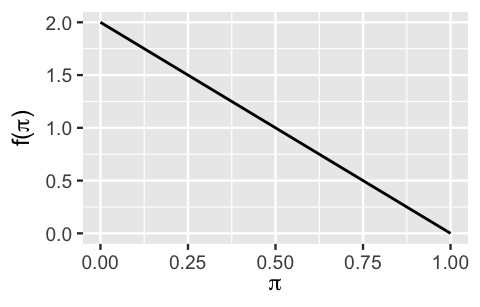

FIGURE 5.2: A conjugate Beta(1,2) prior model for π$\pi$.

5.2 Gamma-Poisson conjugate family

Stop callin’ / Stop callin’ / I don’t wanna think anymore / I got my head and my heart on the dance floor
—Lady Gaga featuring Beyoncé. Lyrics from the song “Telephone.”

Last year, one of this book’s authors got fed up with the number of fraud risk phone calls they were receiving. They set out with a goal of modeling rate λ$\lambda$, the typical number of fraud risk calls received per day. Prior to collecting any data, the author’s guess was that this rate was most likely around 5 calls per day, but could also reasonably range between 2 and 7 calls per day. To learn more, they planned to record the number of fraud risk phone calls on each of n$n$ sampled days, (Y1,Y2,…,Yn)$(Y_1,Y_2,\dots ,Y_n)$.

In moving forward with our investigation of λ$\lambda$, it’s important to recognize that it will not fit into the familiar Beta-Binomial framework. First, λ$\lambda$ is not a proportion limited to be between 0 and 1, but rather a rate parameter that can take on any positive value (e.g., we can’t receive -7 calls per day). Thus, a Beta prior for λ$\lambda$ won’t work. Further, each data point Yi$Y_i$ is a count that can technically take on any non-negative integer in {0,1,2,…}$\{0,1,2,\dots \}$, and thus is not limited by some number of trials n$n$ as is true for the Binomial. Not to fret. Our study of λ$\lambda$ will introduce us to a new conjugate family, the Gamma-Poisson.

5.2.1 The Poisson data model

The spirit of our analysis starts with a prior understanding of λ$\lambda$, the daily rate of fraud risk phone calls. Yet before choosing a prior model structure and tuning this to match our prior understanding, it’s beneficial to identify a model for the dependence of our daily phone call count data Yi$Y_i$ on the typical daily rate of such calls λ$\lambda$. Upon identifying a reasonable data model, we can identify a prior model which can be tuned to match our prior understanding while also mathematically complementing the data model’s corresponding likelihood function. Keeping in mind that each data point Yi$Y_i$ is a random count that can go from 0 to a really big number, Y∈{0,1,2,…}$Y\in \{0,1,2,\dots \}$, the Poisson model, described in its general form below, makes a reasonable candidate for modeling this data.

The Poisson model

Let discrete random variable Y$Y$ be the number of independent events that occur in a fixed amount of time or space, where λ>0$\lambda >0$ is the rate at which these events occur. Then the dependence of Y$Y$ on parameter λ$\lambda$ can be modeled by the Poisson. In mathematical notation:

Y|λ∼Pois(λ).$$Y|\lambda \sim \text{Pois}\left(\lambda \right).$$

Correspondingly, the Poisson model is specified by pmf

f(y|λ)=λye−λy! for y∈{0,1,2,…}$$\begin{array}{}f\left(y|\lambda \right)=\frac{{\lambda }^y{e}^{-\lambda }}{y!}\text{for}y\in \{0,1,2,\dots \}& \text{(5.3)}\end{array}$$

where f(y|λ)$f\left(y|\lambda \right)$ sums to one across y$y$, ∑∞y=0f(y|λ)=1${\sum }_{y=0}^{\infty }f\left(y|\lambda \right)=1$. Further, a Poisson random variable Y$Y$ has equal mean and variance,

E(Y|λ)=Var(Y|λ)=λ.$$\begin{array}{}E\left(Y|\lambda \right)=\text{Var}\left(Y|\lambda \right)=\lambda .& \text{(5.4)}\end{array}$$

Figure 5.3 illustrates the Poisson pmf (5.3) under different rate parameters λ$\lambda$. In general, as the rate of events λ$\lambda$ increases, the typical number of events increases, the variability increases, and the skew decreases. For example, when events occur at a rate of λ=1$\lambda =1$, the model is heavily skewed toward observing a small number of events – we’re most likely to observe 0 or 1 events, and rarely more than 3. In contrast, when events occur at a higher rate of λ=5$\lambda =5$, the model is roughly symmetric and more variable – we’re most likely to observe 4 or 5 events, though have a reasonable chance of observing anywhere between 1 and 10 events.

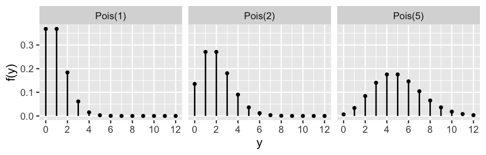
FIGURE 5.3: Poisson pmfs with different rate parameters.

Let (Y1,Y2,…,Yn)$(Y_1,Y_2,\dots ,Y_n)$ denote the number of fraud risk calls we observed on each of the n$n$ days in our data collection period. We assume that the daily number of calls might differ from day to day and can be independently modeled by the Poisson. Thus, on each day i$i$,

Yi|λind∼Pois(λ)$$Y_i|\lambda \stackrel{ind}{\sim }\text{Pois}\left(\lambda \right)$$

with unique pmf

f(yi|λ)=λyie−λyi! for yi∈{0,1,2,…}.$$f\left(y_i|\lambda \right)=\frac{{\lambda }^{y_i}{e}^{-\lambda }}{y_i!}\text{for}{y}_i\in \{0,1,2,\dots \}.$$

Yet in weighing the evidence of the phone call data, we won’t want to analyze each individual day. Rather, we’ll need to process the collective or joint information in our n$n$ data points. This information is captured by the joint probability mass function.

Joint probability mass function

Let (Y1,Y2,…,Yn)$(Y_1,Y_2,\dots ,Y_n)$ be an independent sample of random variables and →y=(y1,y2,…,yn)$\overrightarrow{y}=(y_1,y_2,\dots ,y_n)$ be the corresponding vector of observed values. Further, let f(yi|λ)$f\left(y_i|\lambda \right)$ denote the pmf of an individual observed data point Yi=yi$Y_i=y_i$. Then by the assumption of independence, the following joint pmf specifies the randomness in and plausibility of the collective sample:

f(→y|λ)=n∏i=1f(yi|λ)=f(y1|λ)⋅f(y2|λ)⋅⋯⋅f(yn|λ).$$\begin{array}{}f\left(\overrightarrow{y}|\lambda \right)=\prod _{i=1}^{n}f\left(y_i|\lambda \right)=f\left(y_1|\lambda \right)\cdot f\left(y_2|\lambda \right)\cdot \cdots \cdot f\left(y_n|\lambda \right).& \text{(5.5)}\end{array}$$

Connecting concepts

This product is analogous to the joint probability of independent events being the product of the marginal probabilities, P(A∩B)=P(A)P(B)$P(A\cap B)=P\left(A\right)P\left(B\right)$.

The joint pmf for our fraud risk call sample follows by applying the general definition (5.5) to our Poisson pmfs. Letting the number of calls on each day i$i$ be yi∈{0,1,2,…}$y_i\in \{0,1,2,\dots \}$,

f(→y|λ)=n∏i=1f(yi|λ)=n∏i=1λyie−λyi!.$$\begin{array}{}f\left(\overrightarrow{y}|\lambda \right)=\prod _{i=1}^{n}f\left(y_i|\lambda \right)=\prod _{i=1}^n\frac{{\lambda }^{y_i}{e}^{-\lambda }}{y_i!}.& \text{(5.6)}\end{array}$$

This looks like a mess, but it can be simplified. In this simplification, it’s important to recognize that we have n$n$ unique data points yi$y_i$, not n$n$ copies of the same data point y$y$. Thus, we need to pay careful attention to the i$i$ subscripts. It follows that

f(→y|λ)=λy1e−λy1!⋅λy2e−λy2!⋯λyne−λyn!=[λy1λy2⋯λyn][e−λe−λ⋯e−λ]y1!y2!⋯yn!=λ∑yie−nλ∏ni=1yi!$$\begin{array}{cc}f\left(\overrightarrow{y}|\lambda \right)& =\frac{{\lambda }^{y_1}{e}^{-\lambda }}{y_1!}\cdot \frac{{\lambda }^{y_2}{e}^{-\lambda }}{y_2!}\cdots \frac{{\lambda }^{y_n}{e}^{-\lambda }}{y_n!}\\ & =\frac{[{\lambda }^{y_1}{\lambda }^{y_2}\cdots {\lambda }^{y_n}][e^{-\lambda }{e}^{-\lambda }\cdots e^{-\lambda }]}{y_1!y_2!\cdots y_n!}\\ & =\frac{{\lambda }^{\sum y_i}{e}^{-n\lambda }}{{\prod }_{i=1}^n{y}_i!}\end{array}$$

where we’ve simplified the products in the final line by appealing to the properties below.

Simplifying products

Let (x,y,a,b)$(x,y,a,b)$ be a set of constants. Then we can utilize the following facts when simplifying products involving exponents:

xaxb=xa+b and xaya=(xy)a$$\begin{array}{}{x}^a{x}^b=x^{a+b}\text{and}{x}^a{y}^a=(xy{)}^a& \text{(5.7)}\end{array}$$

Once we observe actual sample data, we can flip this joint pmf on its head to define the likelihood function of λ$\lambda$. The Poisson likelihood function is equivalent in formula to the joint pmf f(→y|λ)$f\left(\overrightarrow{y}|\lambda \right)$, yet is a function of λ$\lambda$ which helps us assess the compatibility of different possible λ$\lambda$ values with our observed collection of sample data →y$\overrightarrow{y}$:

L(λ|→y)=λ∑yie−nλ∏ni=1yi!∝λ∑yie−nλ for λ>0.$$\begin{array}{}L\left(\lambda |\overrightarrow{y}\right)=\frac{{\lambda }^{\sum y_i}{e}^{-n\lambda }}{{\prod }_{i=1}^n{y}_i!}\propto {\lambda }^{\sum y_i}{e}^{-n\lambda }\text{for}\lambda >0.& \text{(5.6)}\end{array}$$

It is convenient to represent the likelihood function up to a proportionality constant here, especially since ∏yi!$\prod y_i!$ will be cumbersome to calculate when n$n$ is large, and what we really care about in the likelihood is λ$\lambda$. And when we express the likelihood up to a proportionality constant, note that the sum of the data points (∑yi$\sum y_i$) and the number of data points (n$n$) is all the information that is required from the data. We don’t need to know the value of each individual data point yi$y_i$. Taking this for a spin with real data points later in our analysis will provide some clarity.

5.2.2 Potential priors

The Poisson data model provides one of two key pieces for our Bayesian analysis of λ$\lambda$, the daily rate of fraud risk calls. The other key piece is a prior model for λ$\lambda$. Our original guess was that this rate is most likely around 5 calls per day, but could also reasonably range between 2 and 7 calls per day. In order to tune a prior to match these ideas about λ$\lambda$, we first have to identify a reasonable probability model structure.

Remember here that λ$\lambda$ is a positive and continuous rate, meaning that λ$\lambda$ does not have to be a whole number. Accordingly, a reasonable prior probability model will also have continuous and positive support, i.e., be defined on λ>0$\lambda >0$. There are several named and studied probability models with this property, including the F$F$, Weibull, and Gamma. We don’t dig into all of these in this book. Rather, to make the λ$\lambda$ posterior model construction more straightforward and convenient, we’ll focus on identifying a conjugate prior model.

Suppose we have a random sample of Poisson random variables (Y1,Y2,…,Yn)$(Y_1,Y_2,\dots ,Y_n)$ with likelihood function L(λ|→y)∝λ∑yie−nλ$L\left(\lambda |\overrightarrow{y}\right)\propto {\lambda }^{\sum y_i}{e}^{-n\lambda }$ for λ>0$\lambda >0$. What do you think would provide a convenient conjugate prior model for λ$\lambda$? Why?

1. A “Gamma” model with pdf f(λ)∝λs−1e−rλ$f\left(\lambda \right)\propto {\lambda }^{s-1}{e}^{-r\lambda }$
2. A “Weibull” model with pdf f(λ)∝λs−1e(−rλ)s$f\left(\lambda \right)\propto {\lambda }^{s-1}{e}^{(-r\lambda {)}^s}$
3. A special case of the “F” model with pdf f(λ)∝λs2−1(1+λ)−s$f\left(\lambda \right)\propto {\lambda }^{\frac{s}{2}-1}{(1+\lambda )}^{-s}$

The answer is a. The Gamma model will provide a conjugate prior for λ$\lambda$ when our data has a Poisson model. You might have guessed this from the section title (clever). You might also have guessed this from the shared features of the Poisson likelihood function L(λ|→y)$L\left(\lambda |\overrightarrow{y}\right)$ (5.6) and the Gamma pdf f(λ)$f\left(\lambda \right)$. Both are proportional to

λ◼e−◼λ$${\lambda }^{■}{e}^{-■\lambda }$$

with differing ◼$■$. In fact, we’ll prove that combining the prior and likelihood produces a posterior pdf with this same structure. That is, the posterior will be of the same Gamma model family as the prior. First, let’s learn more about the Gamma model.

5.2.3 Gamma prior

The Gamma & Exponential models

Let λ$\lambda$ be a continuous random variable which can take any positive value, i.e., λ>0$\lambda >0$. Then the variability in λ$\lambda$ might be well modeled by a Gamma model with shape hyperparameter s>0$s>0$ and rate hyperparameter r>0$r>0$:

λ∼Gamma(s,r).$$\lambda \sim \text{Gamma}(s,r).$$

The Gamma model is specified by continuous pdf

f(λ)=rsΓ(s)λs−1e−rλ for λ>0.$$\begin{array}{}f\left(\lambda \right)=\frac{r^s}{\Gamma \left(s\right)}{\lambda }^{s-1}{e}^{-r\lambda }\text{for}\lambda >0.& \text{(5.8)}\end{array}$$

Further, the central tendency and variability in λ$\lambda$ are measured by:

E(λ)=srMode(λ)=s−1r for s≥1Var(λ)=sr2.$$\begin{array}{}\begin{array}{cc}E\left(\lambda \right)& =\frac{s}{r}\\ \text{Mode}\left(\lambda \right)& =\frac{s-1}{r}\text{for}s\ge 1\\ \text{Var}\left(\lambda \right)& =\frac{s}{r^2}.\end{array}& \text{(5.9)}\end{array}$$

The Exponential model is a special case of the Gamma with shape s=1$s=1$, Gamma(1,r)$\text{Gamma}(1,r)$:

λ∼Exp(r).$$\lambda \sim \text{Exp}\left(r\right).$$

Notice that the Gamma model depends upon two hyperparameters, r$r$ and s$s$. Assess your understanding of how these hyperparameters impact the Gamma model properties in the following quiz.³⁷

Figure 5.4 illustrates how different shape and rate hyperparameters impact the Gamma pdf (5.8). Based on these plots:

1. How would you describe the typical behavior of a Gamma(s,r$s,r$) variable λ$\lambda$ when s>r$s>r$ (e.g., Gamma(2,1))?

   1. Right-skewed with a mean greater than 1.
   2. Right-skewed with a mean less than 1.
   3. Symmetric with a mean around 1.

2. Using the same options as above, how would you describe the typical behavior of a Gamma(s,r$s,r$) variable λ$\lambda$ when s<r$s<r$ (e.g., Gamma(1,2))?

3. For which model is there greater variability in the plausible values of λ$\lambda$, Gamma(20,20) or Gamma(20,100)?
   

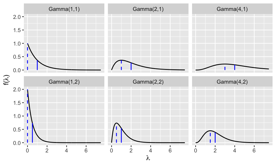
FIGURE 5.4: Gamma models with different hyperparameters. The dashed and solid vertical lines represent the modes and means, respectively.

In general, Figure 5.4 illustrates that λ∼Gamma(s,r)$\lambda \sim \text{Gamma}(s,r)$ variables are positive and right skewed. Further, the general shape and rate of decrease in the skew are controlled by hyperparameters s$s$ and r$r$. The quantitative measures of central tendency and variability in (5.9) provide some insight. For example, notice that the mean of λ$\lambda$, E(λ)=s/r$E\left(\lambda \right)=s/r$, is greater than 1 when s>r$s>r$ and less than 1 when s<r$s<r$. Further, as s$s$ increases relative to r$r$, the skew in λ$\lambda$ decreases and the variability, Var(λ)=s/r2$\text{Var}\left(\lambda \right)=s/r^2$, increases.

Now that we have some intuition for how the Gamma(s,r$s,r$) model works, we can tune it to reflect our prior information about the daily rate of fraud risk phone calls λ$\lambda$. Recall our earlier assumption that λ$\lambda$ is about 5, and most likely somewhere between 2 and 7. Our Gamma(s,r$s,r$) prior should have similar patterns. For example, we want to pick s$s$ and r$r$ for which λ$\lambda$ tends to be around 5,

E(λ)=sr≈5.$$E\left(\lambda \right)=\frac{s}{r}\approx 5.$$

This can be achieved by setting s$s$ to be 5 times r$r$, s=5r$s=5r$. Next we want to make sure that most values of our Gamma(s,r$s,r$) prior are between 2 and 7. Through some trial and error within these constraints, and plotting various Gamma models using plot_gamma() in the bayesrules package, we find that the Gamma(10,2) features closely match the central tendency and variability in our prior understanding (Figure 5.5). Thus, a reasonable prior model for the daily rate of fraud risk phone calls is

λ∼Gamma(10,2)$$\lambda \sim \text{Gamma}(10,2)$$

with prior pdf f(λ)$f\left(\lambda \right)$ following from plugging s=10$s=10$ and r=2$r=2$ into (5.8).

f(λ)=210Γ(10)λ10−1e−2λ for λ>0.$$f\left(\lambda \right)=\frac{2^{10}}{\Gamma \left(10\right)}{\lambda }^{10-1}{e}^{-2\lambda }\text{for}\lambda >0.$$

# Plot the Gamma(10, 2) prior
plot_gamma(shape = 10, rate = 2)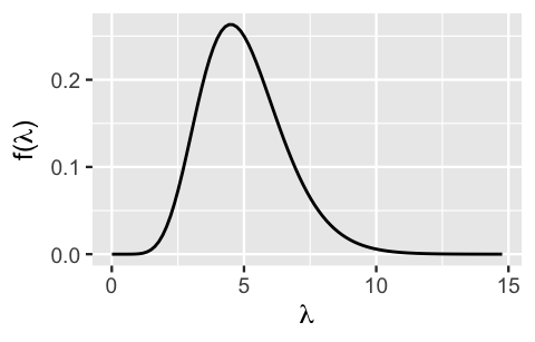

FIGURE 5.5: The pdf of a Gamma(10,2) prior for λ$\lambda$, the daily rate of fraud risk calls.

5.2.4 Gamma-Poisson conjugacy

As we discussed at the start of this chapter, conjugate families can come in handy. Fortunately for us, using a Gamma prior for a rate parameter λ$\lambda$ and a Poisson model for corresponding count data Y$Y$ is another example of a conjugate family. This means that, spoiler, the posterior model for λ$\lambda$ will also have a Gamma model with updated parameters. We’ll state and prove this in the general setting before applying the results to our phone call situation.

The Gamma-Poisson Bayesian model

Let λ>0$\lambda >0$ be an unknown rate parameter and (Y1,Y2,…,Yn)$(Y_1,Y_2,\dots ,Y_n)$ be an independent Pois(λ)$\text{Pois}\left(\lambda \right)$ sample. The Gamma-Poisson Bayesian model complements the Poisson structure of data Y$Y$ with a Gamma prior on λ$\lambda$:

Yi|λind∼Pois(λ)λ∼Gamma(s,r).$$\begin{array}{cc}{Y}_i|\lambda & \stackrel{ind}{\sim }\text{Pois}\left(\lambda \right)\\ \lambda & \sim \text{Gamma}(s,r).\end{array}$$

Upon observing data →y=(y1,y2,…,yn)$\overrightarrow{y}=(y_1,y_2,\dots ,y_n)$, the posterior model of λ$\lambda$ is also a Gamma with updated parameters:

λ|→y∼Gamma(s+∑yi,r+n).$$\begin{array}{}\lambda |\overrightarrow{y}\sim \text{Gamma}(s+\sum y_i,r+n).& \text{(5.10)}\end{array}$$

Let’s prove this result. In general, recall that the posterior pdf of λ$\lambda$ is proportional to the product of the prior pdf and likelihood function defined by (5.8) and (5.6), respectively:

f(λ|→y)∝f(λ)L(λ|→y)=rsΓ(s)λs−1e−rλ⋅λ∑yie−nλ∏yi! for λ>0.$$f\left(\lambda |\overrightarrow{y}\right)\propto f\left(\lambda \right)L\left(\lambda |\overrightarrow{y}\right)=\frac{r^s}{\Gamma \left(s\right)}{\lambda }^{s-1}{e}^{-r\lambda }\cdot \frac{{\lambda }^{\sum y_i}{e}^{-n\lambda }}{\prod y_i!}\text{for}\lambda >0.$$

Next, remember that any non-λ$\lambda$ multiplicative constant in the above equation can be “proportional-ed” out. Thus, boiling the prior pdf and likelihood function down to their kernels, we get

f(λ|→y)∝λs−1e−rλ⋅λ∑yie−nλ=λs+∑yi−1e−(r+n)λ$$\begin{array}{cc}f\left(\lambda |\overrightarrow{y}\right)& \propto {\lambda }^{s-1}{e}^{-r\lambda }\cdot {\lambda }^{\sum y_i}{e}^{-n\lambda }\\ & ={\lambda }^{s+\sum y_i-1}{e}^{-(r+n)\lambda }\end{array}$$

where the final line follows by combining like terms. What we’re left with here is the kernel of the posterior pdf. This particular kernel corresponds to the pdf of a Gamma model (5.8), with shape parameter s+∑yi$s+\sum y_i$ and rate parameter r+n$r+n$. Thus, we’ve proven that

λ|→y∼Gamma(s+∑yi,r+n).$$\lambda |\overrightarrow{y}\sim \text{Gamma}(s+\sum y_i,r+n).$$

Let’s apply this result to our fraud risk calls. There we have a Gamma(10,2) prior for λ$\lambda$, the daily rate of calls. Further, on four separate days in the second week of August, we received →y=(y1,y2,y3,y4)=(6,2,2,1)$\overrightarrow{y}=(y_1,y_2,y_3,y_4)=(6,2,2,1)$ such calls. Thus, we have a sample of n=4$n=4$ data points with a total of 11 fraud risk calls and an average of 2.75 phone calls per day:

4∑i=1yi=6+2+2+1=11 and ¯y=∑4i=1yi4=2.75.$$\sum _{i=1}^4{y}_i=6+2+2+1=11\text{and}\overline{y}=\frac{{\sum }_{i=1}^4{y}_i}{4}=2.75.$$

Plugging this data into (5.6), the resulting Poisson likelihood function of λ$\lambda$ is

L(λ|→y)=λ11e−4λ6!×2!×2!×1!∝λ11e−4λ for λ>0.$$L\left(\lambda |\overrightarrow{y}\right)=\frac{{\lambda }^{11}{e}^{-4\lambda }}{6!\times 2!\times 2!\times 1!}\propto {\lambda }^{11}{e}^{-4\lambda }\text{for}\lambda >0.$$

We visualize a portion of L(λ|→y)$L\left(\lambda |\overrightarrow{y}\right)$ for λ$\lambda$ between 0 and 10 using the plot_poisson_likelihood() function in the bayesrules package. Here, y is the vector of data values and lambda_upper_bound is the maximum value of λ$\lambda$ to view on the x-axis. (Why can’t we visualize the whole likelihood? Because λ∈(0,∞)$\lambda \in (0,\infty )$ and this book would be pretty expensive if we had infinite pages.)

plot_poisson_likelihood(y = c(6, 2, 2, 1), lambda_upper_bound = 10)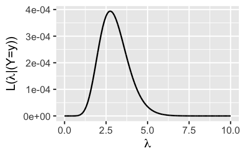

FIGURE 5.6: The likelihood function of λ$\lambda$, the daily rate of fraud risk calls, given a four-day sample of phone call data.

The punchline is this. Underlying rates λ$\lambda$ of between one to five fraud risk calls per day are consistent with our phone call data. And across this spectrum, rates near 2.75 are the most compatible with this data. This makes sense. The Poisson data model assumes that λ$\lambda$ is the underlying average daily phone call count, E(Yi|λ)=λ$E\left(Y_i|\lambda \right)=\lambda$. As such, we’re most likely to observe a sample with an average daily phone call rate of ¯y=2.75$\overline{y}=2.75$ when the underlying rate λ$\lambda$ is also 2.75.

Combining these observations with our Gamma(10,2) prior model of λ$\lambda$, it follows from (5.10) that the posterior model of λ$\lambda$ is a Gamma with an updated shape parameter of 21 (s+∑yi=10+11$s+\sum y_i=10+11$) and rate parameter of 6 (r+n=2+4$r+n=2+4$):

λ|→y∼Gamma(21,6).$$\lambda |\overrightarrow{y}\sim \text{Gamma}(21,6).$$

We can visualize the prior pdf, scaled likelihood function, and posterior pdf for λ$\lambda$ all in a single plot with the plot_gamma_poisson() function in the bayesrules package. How magical. For this function to work, we must specify a few things: the prior shape and rate hyperparameters as well as the information from our data, the observed total number of phone calls sum_y (∑yi)$(\sum y_i)$ and the sample size n:

plot_gamma_poisson(shape = 10, rate = 2, sum_y = 11, n = 4)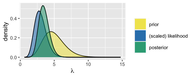

FIGURE 5.7: The Gamma-Poisson model of λ$\lambda$, the daily rate of fraud risk calls.

Our posterior notion about the daily rate of fraud calls is, of course, a compromise between our vague prior and the observed phone call data. Since our prior notion was quite variable in comparison to the strength in our sample data, the posterior model of λ$\lambda$ is more in sync with the data. Specifically, utilizing the properties of the Gamma(10,2) prior and Gamma(21,6) posterior as defined by (5.9), notice that our posterior understanding of the typical daily rate of phone calls dropped from 5 to 3.5 per day:

E(λ)=102=5 and E(λ|→y)=216=3.5.$$E\left(\lambda \right)=\frac{10}{2}=5\text{and}E\left(\lambda |\overrightarrow{y}\right)=\frac{21}{6}=3.5.$$

Though a compromise between the prior mean and data mean, this posterior mean is closer to the data mean of ¯y=2.75$\overline{y}=2.75$ calls per day.

Hot tip

The posterior mean will always be between the prior mean and the data mean. If your posterior mean falls outside that range, it indicates that you made an error and should retrace some steps.

Further, with the additional information about λ$\lambda$ from the data, the variability in our understanding of λ$\lambda$ drops by more than half, from a standard deviation of 1.581 to 0.764 calls per day:

SD(λ)=√1022=1.581 and SD(λ|→y)=√2162=0.764.$$\text{SD}\left(\lambda \right)=\sqrt{\frac{10}{2^2}}=1.581\text{and}\text{SD}\left(\lambda |\overrightarrow{y}\right)=\sqrt{\frac{21}{6^2}}=0.764.$$

The convenient summarize_gamma_poisson() function in the bayesrules package, which uses the same arguments as plot_gamma_poisson(), helps us contrast the prior and posterior models and confirms the results above:

summarize_gamma_poisson(shape = 10, rate = 2, sum_y = 11, n = 4)
      model shape rate mean  mode    var     sd
1     prior    10    2  5.0 4.500 2.5000 1.5811
2 posterior    21    6  3.5 3.333 0.5833 0.7638

5.3 Normal-Normal conjugate family

We now have two conjugate families in our toolkit: the Beta-Binomial and the Gamma-Poisson. But many more conjugate families exist! It’s impossible to cover them all, but there is a third conjugate family that’s especially helpful to know: the Normal-Normal. Consider a data story. As scientists learn more about brain health, the dangers of concussions (hence of activities in which participants sustain repeated concussions) are gaining greater attention (Bachynski 2019). Among all people who have a history of concussions, we are interested in μ$\mu$, the average volume (in cubic centimeters) of a specific part of the brain: the hippocampus. Though we don’t have prior information about this group in particular, Wikipedia tells us that among the general population of human adults, both halves of the hippocampus have a volume between 3.0 and 3.5 cubic centimeters.³⁸ Thus, the total hippocampal volume of both sides of the brain is between 6 and 7 cm3${\text{cm}}^3$. Using this as a starting point, we’ll assume that the mean hippocampal volume among people with a history of concussions, μ$\mu$, is also somewhere between 6 and 7 cm3${\text{cm}}^3$, with an average of 6.5. We’ll balance this prior understanding with data on the hippocampal volumes of n=25$n=25$ subjects, (Y1,Y2,…,Yn)$(Y_1,Y_2,\dots ,Y_n)$, using the Normal-Normal Bayesian model.

5.3.1 The Normal data model

Again, the spirit of our Bayesian analysis starts with our prior understanding of μ$\mu$. Yet the specification of an appropriate prior model structure for μ$\mu$ (which we can then tune) can be guided by first identifying a model for the dependence of our data Yi$Y_i$ upon μ$\mu$. Since hippocampal volumes Yi$Y_i$ are measured on a continuous scale, there are many possible common models of the variability in Yi$Y_i$ from person to person: Beta, Exponential, Gamma, Normal, F, etc. From this list, we can immediately eliminate the Beta model – it assumes that Yi∈[0,1]$Y_i\in [0,1]$, whereas hippocampal volumes tend to be around 6.5 cm3${\text{cm}}^3$. Among the remaining options, the Normal model is quite reasonable – biological measurements like hippocampal volume are often symmetrically or Normally distributed around some global average, here μ$\mu$.

The Normal model

Let Y$Y$ be a continuous random variable which can take any value between −∞$-\infty$ and ∞$\infty$, i.e., Y∈(−∞,∞)$Y\in (-\infty ,\infty )$. Then the variability in Y$Y$ might be well represented by a Normal model with mean parameter μ∈(−∞,∞)$\mu \in (-\infty ,\infty )$ and standard deviation parameter σ>0$\sigma >0$:

Y∼N(μ,σ2).$$Y\sim N(\mu ,{\sigma }^2).$$

The Normal model is specified by continuous pdf

f(y)=1√2πσ2exp[−(y−μ)22σ2] for y∈(−∞,∞)$$\begin{array}{}f\left(y\right)=\frac{1}{\sqrt{2\pi {\sigma }^2}}\exp [-\frac{(y-\mu {)}^2}{2{\sigma }^2}]\text{for}y\in (-\infty ,\infty )& \text{(5.11)}\end{array}$$

and has the following features:

E(Y)= Mode(Y)=μVar(Y)=σ2SD(Y)=σ.$$\begin{array}{cc}E\left(Y\right)& =\text{Mode}\left(Y\right)=\mu \\ \text{Var}\left(Y\right)& ={\sigma }^2\\ \text{SD}\left(Y\right)& =\sigma .\end{array}$$

Further, σ$\sigma$ provides a sense of scale for Y$Y$. Roughly 95% of Y$Y$ values will be within 2 standard deviations of μ$\mu$:

μ±2σ.$$\begin{array}{}\mu \pm 2\sigma .& \text{(5.12)}\end{array}$$

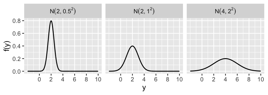
FIGURE 5.8: Normal pdfs with varying mean and standard deviation parameters.

Figure 5.8 illustrates the Normal model under a variety of mean and standard deviation parameter values, μ$\mu$ and σ$\sigma$. No matter the parameters, the Normal model is bell-shaped and symmetric around μ$\mu$ – thus as μ$\mu$ gets larger, the model shifts to the right along with it. Further, σ$\sigma$ controls the variability of the Normal model – as σ$\sigma$ gets larger, the model becomes more spread out. Finally, though a Normal variable Y$Y$ can technically range from −∞$-\infty$ to ∞$\infty$, the Normal model assigns negligible plausibility to Y$Y$ values that are more than 3 standard deviations σ$\sigma$ from the mean μ$\mu$. To play around some more, you can plot Normal models using the plot_normal() function from the bayesrules package.

Returning to our brain analysis, we can reasonably assume that the hippocampal volumes of our n=25$n=25$ subjects, (Y1,Y2,…,Yn)$(Y_1,Y_2,\dots ,Y_n)$, are independent and Normally distributed around a mean volume μ$\mu$ with standard deviation σ$\sigma$. Further, to keep our focus on μ$\mu$, we’ll assume throughout our analysis that the standard deviation is known to be σ=0.5$\sigma =0.5$ cm3${\text{cm}}^3$.³⁹ This choice of σ$\sigma$ suggests that most people have hippocampal volumes within 2σ=1$2\sigma =1$ cm3${\text{cm}}^3$ of the average. Thus, the dependence of Yi$Y_i$ on the unknown mean μ$\mu$ is:

Yi|μ∼N(μ,σ2).$$Y_i|\mu \sim N(\mu ,{\sigma }^2).$$

Reasonable doesn’t mean perfect. Though we’ll later see that our hippocampal volume data does exhibit Normal behavior, the Normal model technically assumes that each subject’s hippocampal volume can range from −∞$-\infty$ to ∞$\infty$. However, we’re not too worried about this incorrect assumption here. Per our earlier discussion of Figure 5.8, the Normal model will put negligible weight on unreasonable values of hippocampal volume. In general, not letting perfect be the enemy of good will be a theme throughout this book (mainly because there is no perfect).

Accordingly, the joint pdf which describes the collective randomness in our n=25$n=25$ subjects’ hippocampal volumes, (Y1,Y2,…,Yn)$(Y_1,Y_2,\dots ,Y_n)$, is the product of the unique Normal pdfs f(yi|μ)$f\left(y_i|\mu \right)$ defined by (5.11),

f(→y|μ)=n∏i=1f(yi|μ)=n∏i=11√2πσ2exp[−(yi−μ)22σ2].$$f\left(\overrightarrow{y}|\mu \right)=\prod _{i=1}^{n}f\left(y_i|\mu \right)=\prod _{i=1}^n\frac{1}{\sqrt{2\pi {\sigma }^2}}\exp [-\frac{(y_i-\mu {)}^2}{2{\sigma }^2}].$$

Once we observe our sample data →y$\overrightarrow{y}$, we can flip the joint pdf on its head to obtain the Normal likelihood function of μ$\mu$, L(μ|→y)=f(→y|μ)$L\left(\mu |\overrightarrow{y}\right)=f\left(\overrightarrow{y}|\mu \right)$. Remembering that we’re assuming σ$\sigma$ is a known constant, we can simplify the likelihood up to a proportionality constant by dropping the terms that don’t depend upon μ$\mu$. Then for μ∈(−∞,∞)$\mu \in (-\infty ,\infty )$,

L(μ|→y)∝n∏i=1exp[−(yi−μ)22σ2]=exp[−∑ni=1(yi−μ)22σ2].$$L\left(\mu |\overrightarrow{y}\right)\propto \prod _{i=1}^n\exp [-\frac{(y_i-\mu {)}^2}{2{\sigma }^2}]=\exp [-\frac{{\sum }_{i=1}^n(y_i-\mu {)}^2}{2{\sigma }^2}].$$ Through a bit more rearranging (which we encourage you to verify if, like us, you enjoy algebra), we can make this even easier to digest by using the sample mean ˉy$\overline{y}$ and sample size n$n$ to summarize our data values:

L(μ|→y)∝exp[−(ˉy−μ)22σ2/n] for μ∈(−∞,∞).$$\begin{array}{}L\left(\mu |\overrightarrow{y}\right)\propto \exp [-\frac{(\overline{y}-\mu {)}^2}{2{\sigma }^2/n}]\text{for}\mu \in (-\infty ,\infty ).& \text{(5.13)}\end{array}$$

Don’t forget the whole point of this exercise! Specifying a model for the data along with its corresponding likelihood function provides the tools we’ll need to assess the compatibility of our data →y$\overrightarrow{y}$ with different values of μ$\mu$ (once we actually collect that data).

5.3.2 Normal prior

With the likelihood in place, let’s formalize a prior model for μ$\mu$, the mean hippocampal volume among people that have a history of concussions. By the properties of the Yi|μ∼N(μ,σ2)$Y_i|\mu \sim N(\mu ,{\sigma }^2)$ data model, the Normal mean parameter μ$\mu$ can technically take any value between −∞$-\infty$ and ∞$\infty$. Thus, a Normal prior for μ$\mu$, which is also defined for μ∈(−∞,∞)$\mu \in (-\infty ,\infty )$, makes a reasonable choice. Specifically, we’ll assume that μ$\mu$ itself is Normally distributed around some mean θ$\theta$ with standard deviation τ$\tau$:

μ∼N(θ,τ2),$$\mu \sim N(\theta ,{\tau }^2),$$

where μ$\mu$ has prior pdf

f(μ)=1√2πτ2exp[−(μ−θ)22τ2] for μ∈(−∞,∞).$$\begin{array}{}f\left(\mu \right)=\frac{1}{\sqrt{2\pi {\tau }^2}}\exp [-\frac{(\mu -\theta {)}^2}{2{\tau }^2}]\text{for}\mu \in (-\infty ,\infty ).& \text{(5.14)}\end{array}$$

Not only does the Normal prior assumption that μ∈(−∞,∞)$\mu \in (-\infty ,\infty )$ match the same assumption of the Normal data model, we’ll prove below that this is a conjugate prior. You might anticipate this result from the fact that the likelihood function L(μ|→y)$L\left(\mu |\overrightarrow{y}\right)$ (5.13) and prior pdf f(μ)$f\left(\mu \right)$ (5.14) are both proportional to

exp[−(μ−◼)22◼2]$$\exp [-\frac{(\mu -■{)}^2}{2{■}^2}]$$

with different ◼$■$.

Using our understanding of a Normal model, we can now tune the prior hyperparameters θ$\theta$ and τ$\tau$ to reflect our prior understanding and uncertainty about the average hippocampal volume among people that have a history of concussions, μ$\mu$. Based on our rigorous Wikipedia research that hippocampal volumes tend to be between 6 and 7 cm3${\text{cm}}^3$, we’ll set the Normal prior mean θ$\theta$ to the midpoint, 6.5. Further, we’ll set the Normal prior standard deviation to τ=0.4$\tau =0.4$. In other words, by (5.12), we think there’s a 95% chance that μ$\mu$ is somewhere between 5.7 and 7.3 cm3${\text{cm}}^3$ (6.5±2∗0.4$6.5\pm 2\ast 0.4$). This range is wider, and hence more conservative, than what Wikipedia indicated. Our uncertainty here reflects the fact that we didn’t vet the Wikipedia sources, we aren’t confident that the features for the typical adult translates to people with a history of concussions, and we generally aren’t sure what’s going on here (i.e., we’re not brain experts). Putting this together, our tuned prior model for μ$\mu$ is:

μ∼N(6.5,0.42).$$\mu \sim N(6.5,{0.4}^2).$$

plot_normal(mean = 6.5, sd = 0.4)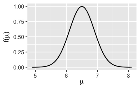

FIGURE 5.9: A Normal prior model for μ$\mu$, with mean 6.5 and standard deviation 0.4.

5.3.3 Normal-Normal conjugacy

To obtain our posterior model of μ$\mu$ we must combine the information from our prior and our data. Again, we were clever to pick a Normal prior model – the Normal-Normal is another convenient conjugate family! Thus, the posterior model for μ$\mu$ will also be Normal with updated parameters that are informed by the prior and observed data.

The Normal-Normal Bayesian model

Let μ∈(−∞,∞)$\mu \in (-\infty ,\infty )$ be an unknown mean parameter and (Y1,Y2,…,Yn)$(Y_1,Y_2,\dots ,Y_n)$ be an independent N(μ,σ2)$N(\mu ,{\sigma }^2)$ sample where σ$\sigma$ is assumed to be known. The Normal-Normal Bayesian model complements the Normal data structure with a Normal prior on μ$\mu$:

Yi|μind∼N(μ,σ2)μ∼N(θ,τ2)$$\begin{array}{cc}{Y}_i|\mu & \stackrel{ind}{\sim }N(\mu ,{\sigma }^2)\\ \mu & \sim N(\theta ,{\tau }^2)\end{array}$$

Upon observing data →y=(y1,y2,…,yn)$\overrightarrow{y}=(y_1,y_2,\dots ,y_n)$ with mean ¯y$\overline{y}$, the posterior model of μ$\mu$ is also Normal with updated parameters:

μ|→y∼N(θσ2nτ2+σ2+ˉynτ2nτ2+σ2,τ2σ2nτ2+σ2).$$\begin{array}{}\mu |\overrightarrow{y}\sim N(\theta \frac{{\sigma }^2}{n{\tau }^2+{\sigma }^2}+\overline{y}\frac{n{\tau }^2}{n{\tau }^2+{\sigma }^2},\frac{{\tau }^2{\sigma }^2}{n{\tau }^2+{\sigma }^2}).& \text{(5.15)}\end{array}$$

Whooo, that is a mouthful! We provide an optional proof of this result in Section 5.3.4. Even without that proof, we can observe the balance that the Normal posterior (5.15) strikes between the prior and the data. First, the posterior mean is a weighted average of the prior mean E(μ)=θ$E\left(\mu \right)=\theta$ and the sample mean ¯y$\overline{y}$. Second, the posterior variance is informed by the prior variability τ$\tau$ and variability in the data σ$\sigma$. Both are impacted by sample size n$n$. First, as n$n$ increases, the posterior mean places less weight on the prior mean and more weight on sample mean ¯y$\overline{y}$:

σ2nτ2+σ2→0 and nτ2nτ2+σ2→1.$$\frac{{\sigma }^2}{n{\tau }^2+{\sigma }^2}\to 0\text{and}\frac{n{\tau }^2}{n{\tau }^2+{\sigma }^2}\to 1.$$

Further, as n$n$ increases, the posterior variance decreases:

τ2σ2nτ2+σ2→0.$$\frac{{\tau }^2{\sigma }^2}{n{\tau }^2+{\sigma }^2}\to 0.$$

That is, the more and more data we have, our posterior certainty about μ$\mu$ increases and becomes more in sync with the data.

Let’s apply and examine this result in our analysis of μ$\mu$, the average hippocampal volume among people that have a history of concussions. We’ve already built our prior model of μ$\mu$, μ∼N(6.5,0.42)$\mu \sim N(6.5,{0.4}^2)$. Next, consider some data. The football data in bayesrules, a subset of the FootballBrain data in the Lock5Data package (Lock et al. 2016), includes results for a cross-sectional study of hippocampal volumes among 75 subjects (Singh et al. 2014): 25 collegiate football players with a history of concussions (fb_concuss), 25 collegiate football players that do not have a history of concussions (fb_no_concuss), and 25 control subjects. For our analysis, we’ll focus on the n=25$n=25$ subjects with a history of concussions (fb_concuss):

# Load the data
data(football)
concussion_subjects <- football %>%
  filter(group == "fb_concuss")

These subjects have an average hippocampal volume of ¯y$\overline{y}$ = 5.735 cm3${\text{cm}}^3$:

concussion_subjects %>%
  summarize(mean(volume))
  mean(volume)
1        5.735

Further, the hippocampal volumes appear to vary normally from subject to subject, ranging from roughly 4.5 to 7 cm3${\text{cm}}^3$. That is, our assumed Normal data model about individual hippocampal volumes, Yi|μ∼N(μ,σ2)$Y_i|\mu \sim N(\mu ,{\sigma }^2)$ with an assumed standard deviation of σ=0.5$\sigma =0.5$, seems reasonable:

ggplot(concussion_subjects, aes(x = volume)) + 
  geom_density()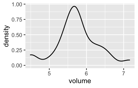

FIGURE 5.10: A density plot of the hippocampal volumes (in cubic centimeters) among 25 subjects that have experienced concussions.

Plugging this information from the data (n=25$n=25$, ¯y$\overline{y}$ = 5.735, and σ=0.5$\sigma =0.5$) into (5.13) defines the Normal likelihood function of μ$\mu$:

L(μ|→y)∝exp[−(5.735−μ)22(0.52/25)] for μ∈(−∞,∞).$$L\left(\mu |\overrightarrow{y}\right)\propto \exp [-\frac{(5.735-\mu {)}^2}{2\left({0.5}^2/25\right)}]\text{for}\mu \in (-\infty ,\infty ).$$

We plot this likelihood function using plot_normal_likelihood(), providing our observed volume data and data standard deviation σ=0.5$\sigma =0.5$ (Figure 5.11). This likelihood illustrates the compatibility of our observed hippocampal data with different μ$\mu$ values. To this end, the hippocampal patterns observed in our data would most likely have arisen if the mean hippocampal volume across all people with a history of concussions, μ$\mu$, were between 5.3 and 6.1 cm3${\text{cm}}^3$. Further, we’re most likely to have observed a mean volume of ¯y=$\overline{y}=$ 5.735 among our 25 sample subjects if the underlying population mean μ$\mu$ were also 5.735.

plot_normal_likelihood(y = concussion_subjects$volume, sigma = 0.5)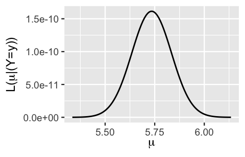

FIGURE 5.11: The Normal likelihood function for mean hippocampal volume μ$\mu$.

We now have all necessary pieces to plug into (5.15), and hence to specify the posterior model of μ$\mu$:

• our Normal prior model of μ$\mu$ had mean θ=6.5$\theta =6.5$ and standard deviation τ=0.4$\tau =0.4$;
• our n=25$n=25$ sample subjects had a sample mean volume ˉy=5.735$\overline{y}=5.735$;
• we assumed a known standard deviation among individual hippocampal volumes of σ=0.5$\sigma =0.5$.

It follows that the posterior model of μ$\mu$ is:

μ|→y∼N(6.5⋅0.5225⋅0.42+0.52+5.735⋅25⋅0.4225⋅0.42+0.52,0.42⋅0.5225⋅0.42+0.52).$$\mu |\overrightarrow{y}\sim N(6.5\cdot \frac{{0.5}^2}{25\cdot {0.4}^2+{0.5}^2}+5.735\cdot \frac{25\cdot {0.4}^2}{25\cdot {0.4}^2+{0.5}^2},\frac{{0.4}^2\cdot {0.5}^2}{25\cdot {0.4}^2+{0.5}^2}).$$

Further simplified,

μ|→y∼N(5.78,0.0092)$$\mu |\overrightarrow{y}\sim N(5.78,{0.009}^2)$$

where the posterior mean places roughly 94% of its weight on the data mean (¯y=5.375$\overline{y}=5.375$) and only 6% of its weight on the prior mean (E(μ)=6.5$E\left(\mu \right)=6.5$):

E(μ|→y)=6.5⋅0.0588+5.735⋅0.9412=5.78.$$E\left(\mu |\overrightarrow{y}\right)=6.5\cdot 0.0588+5.735\cdot 0.9412=5.78.$$

Bringing all of these pieces together, we plot and summarize our Normal-Normal analysis of μ$\mu$ using plot_normal_normal() and summarize_normal_normal() in the bayesrules package. Though a compromise between the prior and data, our posterior understanding of μ$\mu$ is more heavily influenced by the latter. In light of our data, we are much more certain about the mean hippocampal volume among people with a history of concussions, and believe that this figure is somewhere in the range from 5.586 to 5.974 cm3${\text{cm}}^3$ (5.78±2∗0.097$5.78\pm 2\ast 0.097$).

plot_normal_normal(mean = 6.5, sd = 0.4, sigma = 0.5,
                   y_bar = 5.735, n = 25)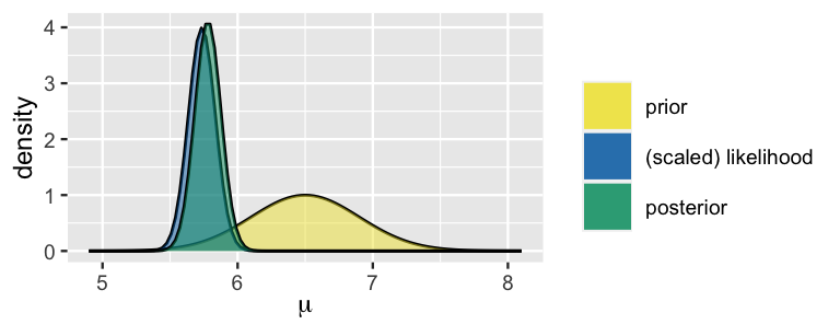

FIGURE 5.12: The Normal-Normal model of μ$\mu$, average hippocampal volume.

summarize_normal_normal(mean = 6.5, sd = 0.4, sigma = 0.5,
                        y_bar = 5.735, n = 25)
      model mean mode      var      sd
1     prior 6.50 6.50 0.160000 0.40000
2 posterior 5.78 5.78 0.009412 0.09701

5.3.4 Optional: Proving Normal-Normal conjugacy

For completeness sake, we prove here that the Normal-Normal model produces posterior model (5.15). If derivations are not your thing, that’s totally fine. Feel free to skip ahead to the next section and know that you can use this Normal-Normal model with a light heart. Let’s get right into it. The posterior pdf of μ$\mu$ is proportional to the product of the Normal prior pdf (5.14) and the likelihood function (5.13). For μ∈(−∞,∞)$\mu \in (-\infty ,\infty )$:

f(μ|→y)∝f(μ)L(μ|→y)∝exp[−(μ−θ)22τ2]⋅exp[−(ˉy−μ)22σ2/n].$$f\left(\mu |\overrightarrow{y}\right)\propto f\left(\mu \right)L\left(\mu |\overrightarrow{y}\right)\propto \exp [\frac{-(\mu -\theta {)}^2}{2{\tau }^2}]\cdot \exp [-\frac{(\overline{y}-\mu {)}^2}{2{\sigma }^2/n}].$$

Next, we can expand the squares in the exponents and sweep under the rug of proportionality both the θ2${\theta }^2$ in the numerator of the first exponent and the ˉy2${\overline{y}}^2$ in the numerator of the second exponent:

f(μ|→y)∝exp[−μ2+2μθ−θ22τ2]exp[−μ2+2μˉy−ˉy22σ2/n]∝exp[−μ2+2μθ2τ2]exp[−μ2+2μˉy2σ2/n].$$\begin{array}{cc}f\left(\mu |\overrightarrow{y}\right)& \propto \exp [\frac{-{\mu }^2+2\mu \theta -{\theta }^2}{2{\tau }^2}]\exp [\frac{-{\mu }^2+2\mu \overline{y}-{\overline{y}}^2}{2{\sigma }^2/n}]\\ & \propto \exp [\frac{-{\mu }^2+2\mu \theta }{2{\tau }^2}]\exp [\frac{-{\mu }^2+2\mu \overline{y}}{2{\sigma }^2/n}].\end{array}$$

Next, we give the exponents common denominators and combine them into a single exponent:

f(μ|→y)∝exp[(−μ2+2μθ)σ2/n2τ2σ2/n]exp[(−μ2+2μˉy)τ22τ2σ2/n]∝exp[(−μ2+2μθ)σ2+(−μ2+2μˉy)nτ22τ2σ2].$$\begin{array}{cc}f\left(\mu |\overrightarrow{y}\right)& \propto \exp [\frac{(-{\mu }^2+2\mu \theta ){\sigma }^2/n}{2{\tau }^2{\sigma }^2/n}]\exp [\frac{(-{\mu }^2+2\mu \overline{y}){\tau }^2}{2{\tau }^2{\sigma }^2/n}]\\ & \propto \exp [\frac{(-{\mu }^2+2\mu \theta ){\sigma }^2+(-{\mu }^2+2\mu \overline{y})n{\tau }^2}{2{\tau }^2{\sigma }^2}].\end{array}$$

Now let’s combine μ$\mu$ terms and rearrange so that μ2${\mu }^2$ is by itself:

f(μ|→y)∝exp[−μ2(nτ2+σ2)+2μ(θσ2+ˉynτ2)2τ2σ2]∝exp[−μ2+2μ(θσ2+ˉynτ2nτ2+σ2)2(τ2σ2)/(nτ2+σ2)].$$\begin{array}{cc}f\left(\mu |\overrightarrow{y}\right)& \propto \exp [\frac{-{\mu }^2(n{\tau }^2+{\sigma }^2)+2\mu (\theta {\sigma }^2+\overline{y}n{\tau }^2)}{2{\tau }^2{\sigma }^2}]\\ & \propto \exp [\frac{-{\mu }^2+2\mu \left(\frac{\theta {\sigma }^2+\overline{y}n{\tau }^2}{n{\tau }^2+{\sigma }^2}\right)}{2\left({\tau }^2{\sigma }^2\right)/(n{\tau }^2+{\sigma }^2)}].\end{array}$$

This may seem like too much to deal with, but if you look closely, you can see that we can bring back some constants which do not depend upon μ$\mu$ to complete the square in the numerator:

f(μ|→y)∝exp[−(μ−θσ2+ˉynτ2nτ2+σ2)22(τ2σ2)/(nτ2+σ2)].$$\begin{array}{cc}f\left(\mu |\overrightarrow{y}\right)& \propto \exp [\frac{-(\mu -\frac{\theta {\sigma }^2+\overline{y}n{\tau }^2}{n{\tau }^2+{\sigma }^2}{)}^2}{2\left({\tau }^2{\sigma }^2\right)/(n{\tau }^2+{\sigma }^2)}].\end{array}$$

This may still seem messy, but once we complete the square, we actually have the kernel of a Normal pdf for μ$\mu$, exp[−(μ−◼)22◼2]$\exp [-\frac{(\mu -■{)}^2}{2{■}^2}]$. By identifying the missing pieces ◼$■$, we can thus conclude that

μ|→y∼N(θσ2+ˉynτ2nτ2+σ2,τ2σ2nτ2+σ2)$$\mu |\overrightarrow{y}\sim N(\frac{\theta {\sigma }^2+\overline{y}n{\tau }^2}{n{\tau }^2+{\sigma }^2},\frac{{\tau }^2{\sigma }^2}{n{\tau }^2+{\sigma }^2})$$

where we can reorganize the posterior mean as a weighted average of the prior mean μ$\mu$ and data mean ¯y$\overline{y}$:

θσ2+ˉynτ2nτ2+σ2=θσ2nτ2+σ2+ˉynτ2nτ2+σ2.$$\frac{\theta {\sigma }^2+\overline{y}n{\tau }^2}{n{\tau }^2+{\sigma }^2}=\theta \frac{{\sigma }^2}{n{\tau }^2+{\sigma }^2}+\overline{y}\frac{n{\tau }^2}{n{\tau }^2+{\sigma }^2}.$$

5.4 Why no simulation in this chapter?

As you may have gathered, we love some simulations. There is something reassuring about the reality check that a simulation can provide. Yet we are at a crossroads. The Gamma-Poisson and Normal-Normal models we’ve studied here are tough to simulate using the techniques we’ve learned thus far. Letting θ$\theta$ represent some parameter of interest, recall the steps we’ve used for past simulations:

1. Simulate, say, 10000 values of θ$\theta$ from the prior model.
2. Simulate a set of sample data Y$Y$ from each simulated θ$\theta$ value.
3. Filter out only those of the 10000 simulated sets of (θ,Y)$(\theta ,Y)$ for which the simulated Y$Y$ data matches the data we actually observed.
4. Use the remaining θ$\theta$ values to approximate the posterior of θ$\theta$.

The issue with extending this simulation technique to the Gamma-Poisson and Normal-Normal examples in this chapter comes with step 3. In both of our examples, we had a sample size greater than one, (Y1,Y2,…,Yn)$(Y_1,Y_2,\dots ,Y_n)$. Further, in the Normal-Normal example, our data values Yi$Y_i$ are continuous. In both of these scenarios, it’s very likely that no simulated sets of (θ,Y)$(\theta ,Y)$ will perfectly match our observed sample data. This is true even if we carry out millions of simulations in step 3. Spoiler alert! There are other ways to approximate the posterior model which we will learn in Unit 2.

5.5 Critiques of conjugate family models

Before we end the chapter, we want to acknowledge that conjugate family models also have drawbacks. In particular:

• A conjugate prior model isn’t always flexible enough to fit your prior understanding. For example, a Normal model is always unimodal and symmetric around the mean μ$\mu$. So if your prior understanding is not symmetric or is not unimodal, then the Normal prior might not be the best tool for the job.
• Conjugate family models do not always allow you to have an entirely flat prior. While we can tune a flat Beta prior by setting α=β=1$\alpha =\beta =1$, neither the Normal nor Gamma priors (or any proper models with infinite support) can be tuned to be totally flat. The best we can do is tune the priors to have very high variance, so that they’re almost flat.

5.6 Chapter summary

In Chapter 5, you learned about conjugacy and applied it to a few different situations. Our main takeaways for this chapter are:

• Using conjugate priors allows us to have easy-to-derive and readily interpretable posterior models.
• The Beta-Binomial, Gamma-Poisson, and Normal-Normal conjugate families allow us to analyze data Y$Y$ in different scenarios. The Beta-Binomial is convenient when our data Y$Y$ is the number of successes in a set of n$n$ trials, the Gamma-Poisson when Y$Y$ is a count with no upper limit, and the Normal-Normal when Y$Y$ is continuous.
• We can use several functions from the bayesrules package to explore these conjugate families: plot_poisson_likelihood(), plot_gamma(), plot_gamma_poisson(), summarize_gamma_poisson(), plot_normal(), plot_normal_normal(), and summarize_normal_normal().

We hope that you now appreciate the utility of conjugate priors!

5.7 Exercises

5.7.1 Practice: Gamma-Poisson

Exercise 5.1 (Tuning a Gamma prior) For each situation below, tune an appropriate Gamma(s,r$s,r$) prior model for λ$\lambda$.

1. The most common value of λ$\lambda$ is 4, and the mean is 7.
2. The most common value of λ$\lambda$ is 10 and the mean is 12.
3. The most common value of λ$\lambda$ is 5, and the variance is 3.
4. The most common value of λ$\lambda$ is 14, and the variance is 6.
5. The mean of λ$\lambda$ is 4 and the variance is 12.
6. The mean of λ$\lambda$ is 22 and the variance is 3.

Exercise 5.2 (Poisson likelihood functions) For each situation below, we observe the outcomes for a random sample of Poisson variables, Yi|λind∼Pois(λ)$Y_i|\lambda \stackrel{ind}{\sim }\text{Pois}\left(\lambda \right)$. Specify and plot the likelihood function of λ$\lambda$.

1. (y1,y2,y3)=(3,7,19)$(y_1,y_2,y_3)=(3,7,19)$
2. (y1,y2,y3,y4)=(12,12,12,0)$(y_1,y_2,y_3,y_4)=(12,12,12,0)$
3. y1=12$y_1=12$
4. (y1,y2,y3,y4,y5)=(16,10,17,11,11)$(y_1,y_2,y_3,y_4,y_5)=(16,10,17,11,11)$

Exercise 5.3 (Finding the Gamma-Poisson posterior) Assume a prior model of λ∼Gamma(24,2)$\lambda \sim \text{Gamma}(24,2)$. Specify the posterior models of λ$\lambda$ corresponding to the data in each scenario of Exercise 5.2.

Exercise 5.4 (Finding the Gamma-Poisson posterior with a different prior) Assume a prior model of λ∼Gamma(2,2)$\lambda \sim \text{Gamma}(2,2)$. Specify the posterior models of λ$\lambda$ corresponding to the data in each scenario of Exercise 5.2.

Exercise 5.5 (Text messages) Let random variable λ$\lambda$ represent the rate of text messages people receive in an hour. At first, you believe that the typical number of messages per hour is 5 with a standard deviation of 0.25 messages.

1. Tune and plot an appropriate Gamma(s,r$s,r$) prior model for λ$\lambda$.
2. What is the prior probability that the rate of text messages per hour is larger than 10? Hint: learn about pgamma().

Exercise 5.6 (Text messages with data) Continuing with Exercise 5.5, you collect data from six friends. They received 7, 3, 8, 9, 10, 12 text messages in the previous hour.

1. Plot the resulting likelihood function of λ$\lambda$.
2. Plot the prior pdf, likelihood function, and the posterior pdf of λ$\lambda$.
3. Use summarize_gamma_poisson() to calculate descriptive statistics for the prior and the posterior models of λ$\lambda$.
4. Comment on how your understanding about λ$\lambda$ changed from the prior (in the previous exercise) to the posterior based on the data you collected from your friends.

Exercise 5.7 (World Cup) Let λ$\lambda$ be the average number of goals scored in a Women’s World Cup game. We’ll analyze λ$\lambda$ by the following Gamma-Poisson model where data Yi$Y_i$ is the observed number of goals scored in a sample of World Cup games:

Yi|λind∼Pois(λ)λ∼Gamma(1,0.25)$$\begin{array}{cc}{Y}_i|\lambda & \stackrel{ind}{\sim }\text{Pois}\left(\lambda \right)\\ \lambda & \sim \text{Gamma}(1,0.25)\end{array}$$

1. Plot and summarize our prior understanding of λ$\lambda$.

2. Why is the Poisson model a reasonable choice for our data Yi$Y_i$?

3. The wwc_2019_matches data in the fivethirtyeight package includes the number of goals scored by the two teams in each 2019 Women’s World Cup match. Define, plot, and discuss the total number of goals scored per game:

   library(fivethirtyeight)
   data("wwc_2019_matches")
   wwc_2019_matches <- wwc_2019_matches %>% 
     mutate(total_goals = score1 + score2)

4. Identify the posterior model of λ$\lambda$ and verify your answer using summarize_gamma_poisson().

5. Plot the prior pdf, likelihood function, and posterior pdf of λ$\lambda$. Describe the evolution in your understanding of λ$\lambda$ from the prior to the posterior.

5.7.2 Practice: Normal-Normal

Exercise 5.8 (Normal likelihood functions) In each situation below, we observe the outcomes for a Normal random sample, Yi|μind∼N(μ,σ2)$Y_i|\mu \stackrel{ind}{\sim }N(\mu ,{\sigma }^2)$ with known σ$\sigma$. Specify and plot the corresponding likelihood function of μ$\mu$.

1. (y1,y2,y3)=(−4.3,0.7,−19.4)$(y_1,y_2,y_3)=(-4.3,0.7,-19.4)$ and σ=10$\sigma =10$
2. (y1,y2,y3,y4)=(−12,1.2,−4.5,0.6)$(y_1,y_2,y_3,y_4)=(-12,1.2,-4.5,0.6)$ and σ=6$\sigma =6$
3. (y1,y2)=(12.4,6.1)$(y_1,y_2)=(12.4,6.1)$ and σ=5$\sigma =5$
4. (y1,y2,y3,y4,y5)=(1.6,0.09,1.7,1.1,1.1)$(y_1,y_2,y_3,y_4,y_5)=(1.6,0.09,1.7,1.1,1.1)$ and σ=0.6$\sigma =0.6$

Exercise 5.9 (Investing in stock) You just bought stock in FancyTech. Let random variable μ$\mu$ be the average dollar amount that your FancyTech stock goes up or down in a one-day period. At first, you believe that μ$\mu$ is 7.2 dollars with a standard deviation of 2.6 dollars.

1. Tune and plot an appropriate Normal prior model for μ$\mu$.
2. According to your plot, does it seem plausible that the FancyTech stock would increase by an average of 7.6 dollars in a day?
3. Does it seem plausible that the FancyTech stock would increase by an average of 4 dollars in a day?
4. What is the prior probability that, on average, the stock price goes down? Hint: pnorm().
5. What is the prior probability that, on average, your stock price goes up by more than 8 dollars per day?

Exercise 5.10 (Investing in stock with data) Continuing with Exercise 5.9, it’s reasonable to assume that the daily changes in FancyTech stock value are Normally distributed around an unknown mean of μ$\mu$ with a known standard deviation of σ=2$\sigma =2$ dollars. On a random sample of 4 days, you observe changes in stock value of -0.7, 1.2, 4.5, and -4 dollars.

1. Plot the corresponding likelihood function of μ$\mu$.
2. Plot the prior pdf, likelihood function, and the posterior pdf for μ$\mu$.
3. Use summarize_normal_normal() to calculate descriptive statistics for the prior and the posterior models.
4. Comment on how your understanding about μ$\mu$ evolved from the prior (in the previous exercise) to the posterior based on the observed data.
5. What is the posterior probability that, on average, the stock price goes down? Hint: pnorm().
6. What is the posterior probability that, on average, your stock price goes up by more than 8 dollars per day?

Exercise 5.11 (Normal-Normal calculation) Prof. Abebe and Prof. Morales both recently finished their PhDs and are teaching their first statistics classes at Bayesian University. Their colleagues told them that the average final exam score across all students, μ$\mu$, varies Normally from year to year with a mean of 80 points and a standard deviation of 4. Further, individual students’ scores Y$Y$ vary Normally around μ$\mu$ with a known standard deviation of 3 points.

1. Prof. Abebe conducts the final exam and observes that his 32 students scored an average of 86 points. Calculate the posterior mean and variance of μ$\mu$ using the data from Prof. Abebe’s class.
2. Prof. Morales conducts the final exam and observes that her 32 students scored an average of 82 points. Calculate the posterior mean and variance of μ$\mu$ using the data from Prof. Morales’ class.
3. Next, use Prof. Abebe and Prof. Morales’ combined exams to calculate the posterior mean and variance of μ$\mu$.

Exercise 5.12 (Control brains) In this chapter we used the Normal-Normal model to analyze the mean hippocampal volume among people who have sustained concussions. In this exercise we will explore the mean volume, μ$\mu$, for people who have not been diagnosed with a concussion. As before, we’ll assume that the hippocampal volumes of individuals in this group, Y$Y$, vary Normally around μ$\mu$ with a standard deviation of σ=0.5$\sigma =0.5$ cubic centimeters. We’ll also start with the same prior as before: μ$\mu$ has a Normal prior with mean θ=6.5$\theta =6.5$ and standard deviation τ=0.4$\tau =0.4$.

1. Use the football data to calculate the sample mean hippocampal volume and sample size of the control subjects who have not been diagnosed with a concussion.
2. Identify the posterior model of μ$\mu$ and verify your answer using summarize_normal_normal().
3. Plot the prior pdf, likelihood function, and posterior pdf of μ$\mu$. Describe the evolution in your understanding of μ$\mu$ from the prior to the posterior.

Exercise 5.13 (Australia) Let μ$\mu$ be the average 3 p.m. temperature in Perth, Australia. Not knowing much about Australian weather, your friend’s prior understanding is that the average temperature is likely around 30 degrees Celsius, though might be anywhere between 10 and 50 degrees Celsius. To learn about μ$\mu$, they plan to analyze 1000 days of temperature data. Letting Yi$Y_i$ denote the 3 p.m. temperature on day i$i$, they’ll assume that daily temperatures vary Normally around μ$\mu$ with a standard deviation of 5 degrees: Yi|μ∼N(μ,52)$Y_i|\mu \sim N(\mu ,5^2)$.

1. Tune and plot a Normal prior for μ$\mu$ that reflects your friend’s understanding.
2. The weather_perth data in the bayesrules package includes 1000 daily observations of 3 p.m. temperatures in Perth (temp3pm). Plot this data and discuss whether it’s reasonable to assume a Normal model for the temperature data.
3. Identify the posterior model of μ$\mu$ and verify your answer using summarize_normal_normal().
4. Plot the prior pdf, likelihood function, and posterior pdf of μ$\mu$. Describe the evolution in your understanding of μ$\mu$ from the prior to the posterior.

Exercise 5.14 (Normal-Normal Simulation)

1. Your friend Alex has read Chapter 4 of this book, but not Chapter 5. Explain to Alex why it’s difficult to simulate a Normal-Normal posterior using the simulation methods we have learned thus far.

2. To prove your point, try (and fail) to simulate the posterior of μ$\mu$ for the following model upon observing a single data point Y=1.1$Y=1.1$:

   Y|μ∼N(μ,12)μ∼N(0,12)$$\begin{array}{cc}Y|\mu & \sim N(\mu ,1^2)\\ \mu & \sim N(0,1^2)\end{array}$$

5.7.3 General practice exercises

Exercise 5.15 (Which model?) Below are kernels for Normal, Poisson, Gamma, Beta, and Binomial models. Identify the appropriate model with specific parameter values.

1. f(θ)∝0.3θ0.716−θ$f\left(\theta \right)\propto {0.3}^{\theta }{0.7}^{16-\theta }$ for θ∈{0,1,2,…,16}$\theta \in \{0,1,2,\dots ,16\}$
2. f(θ)∝1/θ!$f\left(\theta \right)\propto 1/\theta !$ for θ∈{0,1,2,…,∞}$\theta \in \{0,1,2,\dots ,\infty \}$
3. f(θ)∝θ4(1−θ)7$f\left(\theta \right)\propto {\theta }^4(1-\theta {)}^7$ for θ∈[0,1]$\theta \in [0,1]$
4. f(θ)∝e−θ2$f\left(\theta \right)\propto e^{-{\theta }^2}$ for θ∈(−∞,∞)$\theta \in (-\infty ,\infty )$

Exercise 5.16 (Which model: Back for more!) Below are kernels for Normal, Poisson, Gamma, Beta, and Binomial models. Identify the appropriate model with specific parameter values.

1. f(θ)∝e−2θθ15$f\left(\theta \right)\propto e^{-2\theta }{\theta }^{15}$ for θ>0$\theta >0$
2. f(θ)∝e−(θ−12)218$f\left(\theta \right)\propto e^{\frac{-(\theta -12{)}^2}{18}}$ for θ∈(−∞,∞)$\theta \in (-\infty ,\infty )$
3. f(θ)∝0.3θ/θ!$f\left(\theta \right)\propto {0.3}^{\theta }/\theta !$ for θ∈{0,1,2,…,∞}$\theta \in \{0,1,2,\dots ,\infty \}$

Exercise 5.17 (Weighted average) In Section 4.3.2, we expressed the Beta-Binomial posterior mean of proportion π$\pi$ as a weighted average of the prior mean and the observed sample proportion. In Section 5.3.3, we expressed the Normal-Normal posterior mean of μ$\mu$ as a weighted average of the prior mean θ$\theta$ and the observed sample mean ¯y$\overline{y}$. Similarly, express the Gamma-Poisson posterior mean of rate λ$\lambda$, E(λ|→y)$E\left(\lambda |\overrightarrow{y}\right)$, as a weighted average of the prior mean E(λ)$E\left(\lambda \right)$ and sample mean ¯y$\overline{y}$.

Exercise 5.18 (Counting insects) A biologist hires you to study the density of a certain insect in the local region. Their prior idea about θ$\theta$, the number of insects per m2$m^2$ area, is well captured by a Gamma model with an expected value of 0.5 insects per m2$m^2$ and a standard deviation of 0.25 insects per m2$m^2$. You then go out to inspect 20 separate m2$m^2$ areas of a nearby field. You count 3, 2, 5, 1, 2 insects in the first five square meters, and then do not encounter the insect in the next 15m2$15m^2$.

1. What model, Normal or Poisson, should you use to model the dependence of your insect count data on the underlying insect density θ$\theta$? Explain why.
2. Plot the prior pdf, likelihood function, and posterior pdf of insect density θ$\theta$. Comment on whether the posterior model is more in sync with the data or prior. Explain why this makes sense.
3. What is the posterior mean and standard deviation of the insect density?
4. Describe your posterior conclusions in context, in a way that a biologist would find helpful.

Exercise 5.19 (The Beta-Geometric model) Consider the following new Bayesian model:

Y|θ∼Geometric(θ)θ∼Beta(α,β)$$\begin{array}{cc}Y|\theta & \sim \text{Geometric}\left(\theta \right)\\ \theta & \sim \text{Beta}(\alpha ,\beta )\end{array}$$

where the Geometric model has pmf f(y|θ)=θ(1−θ)y−1$f\left(y|\theta \right)=\theta (1-\theta {)}^{y-1}$ for y∈{1,2,…}$y\in \{1,2,\dots \}$.

1. Derive the posterior model for θ$\theta$ given observed data Y=y$Y=y$. If possible, identify the name of the posterior model and its parameters.
2. Is the Beta model a conjugate prior for the Geometric data model?

References

Bachynski, Kathleen. 2019. No Game for Boys to Play: The History of Youth Football and the Origins of a Public Health Crisis. UNC Press Books.

Lock, Robin H, Patti Frazer Lock, Kari Lock Morgan, Eric F Lock, and Dennis F Lock. 2016. Statistics: Unlocking the Power of Data. John Wiley & Sons.

Singh, Rashmi, Timothy B Meier, Rayus Kuplicki, Jonathan Savitz, Ikuko Mukai, LaMont Cavanagh, Thomas Allen, et al. 2014. “Relationship of Collegiate Football Experience and Concussion with Hippocampal Volume and Cognitive Outcomes.” Journal of the American Medical Association 311 (18): 1883–88.

---

37. 1:a, 2:b, 3: Gamma(20,20)↩︎

38. https://en.wikipedia.org/wiki/Hippocampus↩︎

39. You’ll have a chance to relax this silly-ish assumption that we know σ$\sigma$ but don’t know μ$\mu$ in later chapters.↩︎