Chapter 13 Logistic Regression

In Chapter 12 we learned that not every regression is Normal. In Chapter 13, we’ll confront another fact: not every response variable \(Y\) is quantitative. Rather, we might wish to model \(Y\), whether or not a singer wins a Grammy, by their album reviews. Or we might wish to model \(Y\), whether or not a person votes, by their age and political leanings. Across these examples, and in classification settings in general, \(Y\) is categorical. In Chapters 13 and 14 we’ll dig into two classification techniques: Bayesian logistic regression and naive Bayesian classification.

Consider the following data story. Suppose we again find ourselves in Australia, the city of Perth specifically. Located on the southwest coast, Perth experiences dry summers and wet winters. Our goal will be to predict whether or not it will rain tomorrow. That is, we want to model \(Y\), a binary categorical response variable, converted to a 0-1 indicator for convenience:

\[Y = \begin{cases} 1 & \text{ if rain tomorrow} \\ 0 & \text{ otherwise} \\ \end{cases} .\]

Though there are various potential predictors of rain, we’ll consider just three:

\[\begin{split} X_1 & = \text{ today's humidity at 9 a.m. (percent)} \\ X_2 & = \text{ today's humidity at 3 p.m. (percent)} \\ X_3 & = \text{ whether or not it rained today. } \\ \end{split}\]

Our vague prior understanding is that on an average day, there’s a roughly 20% chance of rain. We also have a vague sense that the chance of rain increases when preceded by a day with high humidity or rain itself, but we’re foggy on the rate of this increase. Our eventual goal is to combine this prior understanding with data to model \(Y\) by one or more of the predictors above. Certainly, since \(Y\) is categorical, taking our Normal and Poisson regression hammers to this task would be the wrong thing. In Chapter 13, you will pick up a new tool: the Bayesian logistic regression model for binary response variables \(Y\).

• Build a Bayesian logistic regression model of a binary categorical variable \(Y\) by predictors \(X = (X_1,X_2,...,X_p)\).
• Utilize this model to classify, or predict, the outcome of \(Y\) for a given set of predictor values \(X\).
• Evaluate the quality of this classification technique.

# Load packages
library(bayesrules)
library(rstanarm)
library(bayesplot)
library(tidyverse)
library(tidybayes)
library(broom.mixed)

13.1 Pause: Odds & probability

Before jumping into logistic regression, we’ll pause to review the concept of odds and its relationship to probability. Throughout the book, we’ve used probability \(\pi\) to communicate the uncertainty of a given event of interest (e.g., rain tomorrow). Alternatively, we can cite the corresponding odds of this event, defined by the probability that the event happens relative to the probability that it doesn’t happen:

\[\begin{equation} \text{odds} = \frac{\pi}{1-\pi} . \tag{13.1} \end{equation}\]

Mathematically then, whereas a probability \(\pi\) is restricted to values between 0 and 1, odds can range from 0 on up to infinity. To interpret odds across this range, let \(\pi\) be the probability that it rains tomorrow and consider three different scenarios. If the probability of rain tomorrow is \(\pi = 2/3\), then the probability it doesn’t rain is \(1 - \pi = 1/3\) and the odds of rain are 2:

\[\text{odds of rain } = \frac{2/3}{1-2/3} = 2 .\]

That is, it’s twice as likely to rain than to not rain. If the probability of rain tomorrow is \(\pi = 1/3\), then the probability it doesn’t rain is \(2/3\) and the odds of rain are 1/2:

\[\text{odds of rain } = \frac{1/3}{1-1/3} = \frac{1}{2} .\]

That is, it’s half as likely to rain than to not rain tomorrow. Finally, if the chances of rain or no rain tomorrow are 50-50, then the odds of rain are 1:

\[\text{odds of rain } = \frac{1/2}{1-1/2} = 1 .\]

That is, it’s equally likely to rain or not rain tomorrow. These scenarios illuminate the general principles by which to interpret the odds of an event.

Interpreting odds

Let an event of interest have probability \(\pi \in [0,1]\) and corresponding odds \(\pi / (1-\pi) \in [0, \infty)\). Across this spectrum, comparing the odds to 1 provides perspective on an event’s uncertainty:

• The odds of an event are less than 1 if and only if the event’s chances are less than 50-50, i.e., \(\pi < 0.5\).
• The odds of an event are equal to 1 if and only if the event’s chances are 50-50, i.e., \(\pi = 0.5\).
• The odds of an event are greater than 1 if and only if event’s chances are greater than 50-50, i.e., \(\pi > 0.5\).

Finally, just as we can convert probabilities to odds, we can convert odds to probability by rearranging (13.1):

\[\begin{equation} \pi = \frac{\text{odds}}{1 + \text{odds}} . \tag{13.2} \end{equation}\]

Thus, if we learn that the odds of rain tomorrow are 4 to 1, then there’s an 80% chance of rain:

\[\pi = \frac{4}{1 + 4} = 0.8.\]

13.2 Building the logistic regression model

13.2.1 Specifying the data model

Returning to our rain analysis, let \(Y_i\) be the 0/1 indicator of whether or not it rains tomorrow for any given day \(i\). To begin, we’ll model \(Y_i\) by a single predictor, today’s 9 a.m. humidity level \(X_{i1}\). As noted above, neither the Normal nor Poisson regression models are appropriate for this task. So what is?

What’s an appropriate model structure for data \(Y_i\)?

1. Bernoulli (or, equivalently, Binomial with 1 trial)
2. Gamma
3. Beta

One simple question can help us narrow in on an appropriate model structure for any response variable \(Y_i\): what values can \(Y_i\) take and what probability models assume this same set of values? Here, \(Y_i\) is a discrete variable which can only take two values, 0 or 1. Thus, the Bernoulli probability model is the best candidate for the data. Letting \(\pi_i\) denote the probability of rain on day \(i\),

\[Y_i | \pi_i \sim \text{Bern}(\pi_i)\]

with expected value

\[E(Y_i|\pi_i) = \pi_i.\]

To complete the structure of this Bernoulli data model, we must specify how the expected value of rain \(\pi_i\) depends upon predictor \(X_{i1}\). To this end, the logistic regression model is part of the broader class of generalized linear models highlighted in Section 12.7. Thus, we can identify an appropriate link function of \(\pi_i\), \(g(\cdot)\), that’s linearly related to \(X_{i1}\):

\[g(\pi_i) = \beta_0 + \beta_1 X_{i1} .\]

Keeping in mind the principles that went into building the Poisson regression model, take a quick quiz to reflect upon what \(g(\pi_i)\) might be appropriate.⁶⁰

Let \(\pi_i\) and \(\text{odds}_i = \pi_i / (1-\pi_i)\) denote the probability and corresponding odds of rain tomorrow. What’s a reasonable assumption for the dependence of tomorrow’s rain probability \(\pi_i\) on today’s 9 a.m. humidity \(X_{i1}\)?

1. \(\pi_i = \beta_0 + \beta_1 X_{i1}\)
2. \(\text{odds}_i = \beta_0 + \beta_1 X_{i1}\)
3. \(\log(\pi_i) = \beta_0 + \beta_1 X_{i1}\)
4. \(\log(\text{odds}_i) = \beta_0 + \beta_1 X_{i1}\)

Our goal here is to write the Bernoulli mean \(\pi_i\), or a function of this mean \(g(\pi_i)\), as a linear function of predictor \(X_{i1}\), \(\beta_0 + \beta_1 X_{i1}\). Among the options presented in the quiz above, the first three would be mistakes. Whereas the line defined by \(\beta_0 + \beta_1 X_{i1}\) can span the entire real line, \(\pi_i\) (option a) is limited to values between 0 and 1 and \(\text{odds}_i\) (option b) are limited to positive values. Further, when evaluated at \(\pi_i\) values between 0 and 1, \(\log(\pi_i)\) (option c) is limited to negative values. Among these options, \(\log(\pi_i / (1-\pi_i))\) (option d) is the only option that, like \(\beta_0 + \beta_1 X_{i1}\), spans the entire real line. Thus, the most reasonable option is to assume that \(\pi_i\) depends upon predictor \(X_{i1}\) through the logit link function \(g(\pi_i) = \log(\pi_i / (1-\pi_i))\):

\[\begin{equation} Y_i|\beta_0,\beta_1 \stackrel{ind}{\sim} \text{Bern}(\pi_i) \;\; \text{ with } \;\; \log\left(\frac{\pi_i}{1 - \pi_i}\right) = \beta_0 + \beta_1 X_{i1} . \tag{13.3} \end{equation}\]

That is, we assume that the log(odds of rain) is linearly related to 9 a.m. humidity. To work on scales that are (much) easier to interpret, we can rewrite this relationship in terms of odds and probability, the former following from properties of the log function and the latter following from (13.2):

\[\begin{equation} \frac{\pi_i}{1-\pi_i} = e^{\beta_0 + \beta_1 X_{i1}} \;\;\;\; \text{ and } \;\;\;\; \pi_i = \frac{e^{\beta_0 + \beta_1 X_{i1}}}{1 + e^{\beta_0 + \beta_1 X_{i1}}} . \tag{13.4} \end{equation}\]

There are two key features of these transformations, as illustrated by Figure 13.1. First, the relationships on the odds and probability scales are now represented by nonlinear functions. Further, and fortunately, these transformations preserve the properties of odds (which must be non-negative) and probability (which must be between 0 and 1).

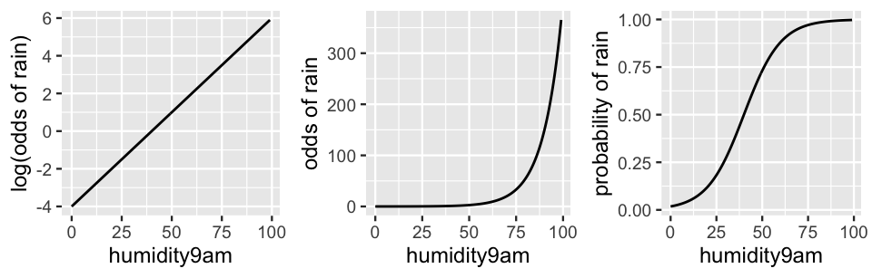
FIGURE 13.1: An example relationship between rain and humidity on the log(odds), odds, and probability scales.

In examining (13.3) and Figure 13.1, notice that parameters \(\beta_0\) and \(\beta_1\) take on the usual intercept and slope meanings when describing the linear relationship between 9 a.m. humidity (\(X_{i1}\)) and the log(odds of rain). Yet the parameter meanings change when describing the nonlinear relationship between 9 a.m. humidity and the odds of rain (13.4). We present a general framework for interpreting logistic regression coefficients here and apply it below.

Interpreting logistic regression coefficients

Let \(Y\) be a binary indicator of some event of interest which occurs with probability \(\pi\). Consider the logistic regression model of \(Y\) with predictors \((X_1,X_2,\ldots,X_p)\):

\[\log(\text{odds}) = \log\left(\frac{\pi}{1-\pi}\right) = \beta_0 + \beta_1 X_1 + \cdots + \beta_p X_p . \]

Interpreting \(\beta_0\)

When \((X_1,X_2,\ldots,X_p)\) are all 0, \(\beta_0\) is the log odds of the event of interest and \(e^{\beta_0}\) is the odds.

Interpreting \(\beta_1\)

When controlling for the other predictors \((X_2,\ldots,X_p)\), let \(\text{odds}_x\) represent the odds of the event of interest when \(X_1 = x\) and \(\text{odds}_{x+1}\) the odds when \(X_1 = x + 1\). Then when \(X_1\) increases by 1, from \(x\) to \(x + 1\), \(\beta_1\) is the typical change in log odds and \(e^{\beta_1}\) is the typical multiplicative change in odds:

\[\beta_1 = \log(\text{odds}_{x+1}) - \log(\text{odds}_x) \;\;\; \text{ and } \;\;\; e^{\beta_1} = \frac{\text{odds}_{x+1}}{\text{odds}_x}.\]

For example, the prior plausible relationship plotted in Figure 13.1 on the log(odds), odds, and probability scales assumes that

\[\log\left(\frac{\pi}{1 - \pi}\right) = -4 + 0.1 X_{i1}.\]

Though humidity levels so close to 0 are merely hypothetical in this area of the world, we extended the plots to the y-axis for perspective on the intercept value \(\beta_0 = -4\). This intercept indicates that on hypothetical days with 0 percent humidity, the log(odds of rain) would be -4. Or, on more meaningful scales, rain would be very unlikely if preceded by a day with 0 humidity:

\[\begin{split} \text{odds of rain } & = e^{-4} = 0.0183 \\ \text{probability of rain } & = \frac{e^{-4}}{1 + e^{-4}} = 0.0180. \\ \end{split}\]

Next, consider the humidity coefficient \(\beta_1 = 0.1\). On the linear log(odds) scale, this is simply the slope: for every one percentage point increase in humidity level, the logged odds of rain increase by 0.1. Huh? This is easier to make sense of on the nonlinear odds scale where the increase is multiplicative. For every one percentage point increase in humidity level, the odds of rain increase by 11%: \(e^{0.1} = 1.11\). Since the probability relationship is a more complicated S-shaped curve, we cannot easily interpret \(\beta_1\) on this scale. However, we can still gather some insights from the probability plot in Figure 13.1. The chance of rain is small when humidity levels hover below 20%, and rapidly increases as humidity levels inch up from 20% to 60%. Beyond 60% humidity, the probability model flattens out near 1, indicating a near certainty of rain.

13.2.2 Specifying the priors

To complete the Bayesian logistic regression model of \(Y\), we must put prior models on our two regression parameters, \(\beta_0\) and \(\beta_1\). As usual, since these parameters can take any value in the real line, Normal priors are appropriate for both. We’ll also assume independence among the priors and express our prior understanding of the model baseline \(\beta_0\) through the centered intercept \(\beta_{0c}\):

\[\begin{equation} \begin{array}{lcrl} \text{data:} & \hspace{.01in} & Y_i|\beta_0,\beta_1 & \stackrel{ind}{\sim} \text{Bern}(\pi_i) \;\; \text{ with } \;\; \log\left(\frac{\pi_i}{1 - \pi_i}\right) = \beta_0 + \beta_1 X_{i1} \\ \text{priors:} & & \beta_{0c} & \sim N\left(-1.4, 0.7^2 \right) \\ & & \beta_1 & \sim N\left(0.07, 0.035^2 \right). \\ \end{array} \tag{13.5} \end{equation}\]

Consider our prior tunings. Starting with the centered intercept \(\beta_{0c}\), recall our prior understanding that on an average day, there’s a roughly 20% chance of rain, i.e., \(\pi \approx 0.2\). Thus, we set the prior mean for \(\beta_{0c}\) on the log(odds) scale to -1.4:

\[\log\left(\frac{\pi}{1-\pi}\right) = \log\left(\frac{0.2}{1-0.2}\right) \approx -1.4 .\]

The range of this Normal prior indicates our vague understanding that the log(odds of rain) might also range from roughly -2.8 to 0 (\(-1.4 \pm 2*0.7\)). More meaningfully, we think that the odds of rain on an average day could be somewhere between 0.06 and 1:

\[\left(e^{-2.8}, e^{0}\right) \approx (0.06, 1)\]

and thus that the probability of rain on an average day could be somewhere between 0.057 and 0.50 (a pretty wide range in the context of rain):

\[\left(\frac{0.06}{1 + 0.06}, \frac{1}{1 + 1}\right) \approx (0.057, 0.50).\]

Next, our prior model on the humidity coefficient \(\beta_1\) reflects our vague sense that the chance of rain increases when preceded by a day with high humidity, but we’re foggy on the rate of this increase and are open to the possibility that it’s nonexistent. Specifically, on the log(odds) scale, we assume that slope \(\beta_1\) ranges somewhere between 0 and 0.14, and is most likely around 0.7. Or, on the odds scale, the odds of rain might increase anywhere from 0% to 15% for every extra percentage point in humidity level:

\[(e^{0}, e^{0.14}) = (1, 1.15) .\]

In originally specifying these priors (before writing them down in the book), we combined a lot of trial and error with an understanding of how logistic regression coefficients work. Throughout this tuning process, we simulated data under a variety of prior models, each time asking ourselves if the results adequately reflected our understanding of rain. To this end, we followed the same framework used in Section 12.1.2 to tune Poisson regression priors.

First, we use the more and more familiar stan_glm() function with prior_PD = TRUE to simulate 20,000 sets of parameters \((\beta_0,\beta_1)\) from the prior models. In doing so, we specify family = binomial to indicate that ours is a logistic regression model with a data structure specified by a Bernoulli / Binomial model (not gaussian or poisson). Even though our model (13.5) doesn’t use default weakly informative priors, and thus no data is used in the prior simulation, stan_glm() still requires that we specify a dataset. Thus, we also load in the weather_perth data from the bayesrules package which contains 1000 days of Perth weather data.⁶¹

# Load and process the data
data(weather_perth)
weather <- weather_perth %>% 
  select(day_of_year, raintomorrow, humidity9am, humidity3pm, raintoday)

# Run a prior simulation
rain_model_prior <- stan_glm(raintomorrow ~ humidity9am,
                             data = weather, family = binomial,
                             prior_intercept = normal(-1.4, 0.7),
                             prior = normal(0.07, 0.035),
                             chains = 4, iter = 5000*2, seed = 84735,
                             prior_PD = TRUE)

Each of the resulting 20,000 prior plausible pairs of \(\beta_0\) and \(\beta_1\) describe a prior plausible relationship between the probability of rain tomorrow and today’s 9 a.m. humidity:

\[\pi = \frac{e^{\beta_0 + \beta_1 X_1}}{1 + e^{\beta_0 + \beta_1 X_1}} .\]

We plot just 100 of these prior plausible relationships below (Figure 13.2 left). These adequately reflect our prior understanding that the probability of rain increases with humidity, as well as our prior uncertainty around the rate of this increase. Beyond this relationship between rain and humidity, we also want to confirm that our priors reflect our understanding of the overall chance of rain in Perth. To this end, we simulate 100 datasets from the prior model. From each dataset (labeled by .draw) we utilize group_by() with summarize() to record the proportion of predicted outcomes \(Y\) (.prediction) that are 1, i.e., the proportion of days on which it rained. Figure 13.2 (right) displays a histogram of these 100 simulated rain rates from our 100 prior simulated datasets. The percent of days on which it rained ranged from as low as roughly 5% in one dataset to as high as roughly 50% in another. This does adequately match our prior understanding and uncertainty about rain in Perth. In contrast, if our prior predictions tended to be centered around high values, we’d question our prior tuning since we don’t believe that Perth is a rainy place.

set.seed(84735)

# Plot 100 prior models with humidity
weather %>% 
  add_fitted_draws(rain_model_prior, n = 100) %>% 
  ggplot(aes(x = humidity9am, y = raintomorrow)) +
    geom_line(aes(y = .value, group = .draw), size = 0.1)

# Plot the observed proportion of rain in 100 prior datasets
weather %>% 
  add_predicted_draws(rain_model_prior, n = 100) %>% 
  group_by(.draw) %>% 
  summarize(proportion_rain = mean(.prediction == 1)) %>% 
  ggplot(aes(x = proportion_rain)) +
    geom_histogram(color = "white")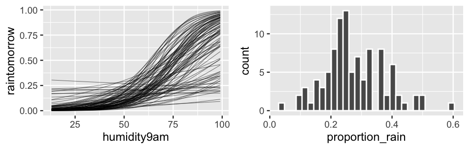

FIGURE 13.2: 100 datasets were simulated from the prior models. For each, we plot the relationship between the probability of rain and the previous day’s humidity level (left) and the observed proportion of days on which it rained (right).

13.3 Simulating the posterior

With the hard work of prior tuning taken care of, consider our data. A visual examination illuminates some patterns in the relationship between rain and humidity. First, a quick jitter plot reveals that rainy days are much less common than non-rainy days. This is especially true at lower humidity levels. Second, though we don’t have enough data to get a stable sense of the probability of rain at each possible humidity level, we can examine the probability of rain on days with similar humidity levels. To this end, we cut() humidity levels into brackets, and then calculate the proportion of days within each bracket that see rain. In general, notice that the chance of rain seems to hover around 10% when humidity levels are below 60%, and then increase from there. This observation is in sync with our prior understanding that rain and humidity are positively associated. However, whereas our prior understanding left open the possibility that the probability of rain might near 100% as humidity levels max out (Figure 13.2), we see in the data that the chance of rain at the highest humidity levels barely breaks 50%.

ggplot(weather, aes(x = humidity9am, y = raintomorrow)) + 
  geom_jitter(size = 0.2)

# Calculate & plot the rain rate by humidity bracket
weather %>% 
  mutate(humidity_bracket = 
           cut(humidity9am, breaks = seq(10, 100, by = 10))) %>% 
  group_by(humidity_bracket) %>% 
  summarize(rain_rate = mean(raintomorrow == "Yes")) %>% 
  ggplot(aes(x = humidity_bracket, y = rain_rate)) + 
    geom_point() + 
    theme(axis.text.x = element_text(angle = 45, vjust = 0.5))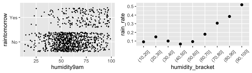

FIGURE 13.3: A jitter plot of rain outcomes versus humidity level (left). A scatterplot of the proportion of days that see rain by humidity bracket (right).

To simulate the posterior model of our logistic regression model parameters \(\beta_0\) and \(\beta_1\) (13.5), we can update() the rain_model_prior simulation in light of this new weather data:\indexfun{update()}

# Simulate the model
rain_model_1 <- update(rain_model_prior, prior_PD = FALSE)

Not that you would forget (!), but we should check diagnostic plots for the stability of our simulation results before proceeding:

# MCMC trace, density, & autocorrelation plots
mcmc_trace(rain_model_1)
mcmc_dens_overlay(rain_model_1)
mcmc_acf(rain_model_1)

We plot 100 posterior plausible models in Figure 13.4. Naturally, upon incorporating the weather data, these models are much less variable than the prior counterparts in Figure 13.2 – i.e., we’re much more certain about the relationship between rain and humidity. We now understand that the probability of rain steadily increases with humidity, yet it’s not until a humidity of roughly 95% that we reach the tipping point when rain becomes more likely than not. In contrast, when today’s 9 a.m. humidity is below 25%, it’s very unlikely to rain tomorrow.

weather %>%
  add_fitted_draws(rain_model_1, n = 100) %>%
  ggplot(aes(x = humidity9am, y = raintomorrow)) +
    geom_line(aes(y = .value, group = .draw), alpha = 0.15) + 
    labs(y = "probability of rain")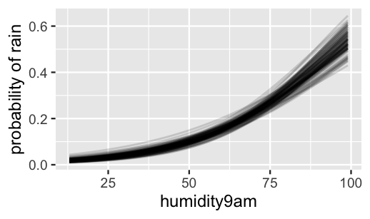

FIGURE 13.4: 100 posterior plausible models for the probability of rain versus the previous day’s humidity level.

More precise information about the relationship between 9 a.m. humidity and rain is contained in the \(\beta_1\) parameter, the approximate posterior model of which is summarized below:

# Posterior summaries on the log(odds) scale
posterior_interval(rain_model_1, prob = 0.80)
                 10%      90%
(Intercept) -5.08785 -4.13450
humidity9am  0.04147  0.05487

# Posterior summaries on the odds scale
exp(posterior_interval(rain_model_1, prob = 0.80))
                 10%     90%
(Intercept) 0.006171 0.01601
humidity9am 1.042339 1.05641

For every one percentage point increase in today’s 9 a.m. humidity, there’s an 80% posterior chance that the log(odds of rain) increases by somewhere between 0.0415 and 0.0549. This rate of increase is less than our 0.07 prior mean for \(\beta_1\) – the chance of rain does significantly increase with humidity, just not to the degree we had anticipated. More meaningfully, for every one percentage point increase in today’s 9 a.m. humidity, the odds of rain increase by somewhere between 4.2% and 5.6%: \((e^{0.0415}, e^{0.0549}) = (1.042, 1.056)\). Equivalently, for every fifteen percentage point increase in today’s 9 a.m. humidity, the odds of rain roughly double: \((e^{15*0.0415}, e^{15*0.0549}) = (1.86, 2.28)\).

13.4 Prediction & classification

Beyond using our Bayesian logistic regression model to better understand the relationship between today’s 9 a.m. humidity and tomorrow’s rain, we also want to predict whether or not it will rain tomorrow. For example, suppose you’re in Perth today and experienced 99% humidity at 9 a.m.. Yuk. To predict whether it will rain tomorrow, we can approximate the posterior predictive model for the binary outcomes of \(Y\), whether or not it rains, where

\[\begin{equation} Y | \beta_0, \beta_1 \sim \text{Bern}(\pi) \;\; \text{ with } \;\; \log\left( \frac{\pi}{1-\pi}\right) = \beta_0 + \beta_1 * 99 . \tag{13.6} \end{equation}\]

To this end, the posterior_predict() function simulates 20,000 rain outcomes \(Y\), one per each of the 20,000 parameter sets in our Markov chain:

# Posterior predictions of binary outcome
set.seed(84735)
binary_prediction <- posterior_predict(
  rain_model_1, newdata = data.frame(humidity9am = 99))

To really connect with the prediction concept, we can also simulate the posterior predictive model from scratch. From each of the 20,000 pairs of posterior plausible pairs of \(\beta_0\) (Intercept) and \(\beta_1\) (humidity9am) in our Markov chain simulation, we calculate the log(odds of rain) (13.6). We then transform the log(odds) to obtain the odds and probability of rain. Finally, from each of the 20,000 probability values \(\pi\), we simulate a Bernoulli outcome of rain, \(Y \sim \text{Bern}(\pi)\), using rbinom() with size = 1:

# Posterior predictions of binary outcome - from scratch
set.seed(84735)
rain_model_1_df <- as.data.frame(rain_model_1) %>% 
  mutate(log_odds = `(Intercept)` + humidity9am*99,
         odds = exp(log_odds),
         prob = odds / (1 + odds),
         Y = rbinom(20000, size = 1, prob = prob))


# Check it out
head(rain_model_1_df, 2)
  (Intercept) humidity9am log_odds   odds   prob Y
1      -4.244     0.04455  0.16577 1.1803 0.5413 0
2      -4.207     0.04210 -0.03934 0.9614 0.4902 1

For example, our first log(odds) and probability values are calculated by plugging \(\beta_0 = -4.244\) and \(\beta_1 = 0.0446\) into (13.6) and transforming it to the probability scale:

\[\begin{split} \log\left( \frac{\pi}{1-\pi}\right) & = -4.244 + 0.0446 * 99 = 0.166 \\ \pi & = \frac{e^{-4.244 + 0.0446 * 99}}{1 + e^{-4.244 + 0.0446 * 99}} = 0.54. \\ \end{split}\]

Subsequently, we randomly draw a binary \(Y\) outcome from the Bern(0.54) model. Though the 0.54 probability of rain in this scenario exceeds 0.5, we ended up observing no rain, \(Y = 0\). Putting all 20,000 predictions together, examine the posterior predictive models of rain obtained from our two methods below. On days with 99% humidity, our Bayesian logistic regression model suggests that rain (\(Y = 1\)) is slightly more likely than not (\(Y = 0\)).

mcmc_hist(binary_prediction) + 
  labs(x = "Y")
ggplot(rain_model_1_df, aes(x = Y)) + 
  stat_count()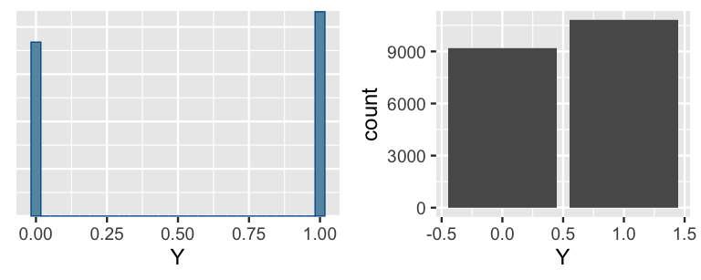

FIGURE 13.5: Posterior predictive model for the incidence of rain using a shortcut function (left) and from scratch (right).

As the name suggests, a common goal in a classification analysis is to turn our observations of the predicted probability of rain (\(\pi\)) or predicted outcome of rain (\(Y\)) into a binary, yes-or-no classification of \(Y\). Take the following quiz to make this classification for yourself.

Suppose it’s 99% humidity at 9 a.m. today. Based on the posterior predictive model above, what binary classification would you make? Will it rain or not? Should we or shouldn’t we carry an umbrella tomorrow?

Questions of classification are somewhat subjective, thus there’s more than one reasonable answer to this quiz. One reasonable answer is this: yes, you should carry an umbrella. Among our 20,000 posterior predictions of \(Y\), 10804 (or 54.02%) called for rain. Thus, since rain was more likely than no rain in the posterior predictive model of \(Y\), it’s reasonable to classify \(Y\) as “1” (rain).

# Summarize the posterior predictions of Y
table(binary_prediction)
binary_prediction
    0     1 
 9196 10804 
colMeans(binary_prediction)
     1 
0.5402 

In making this classification, we used the following classification rule:

• If more than half of our predictions predict \(Y=1\), classify \(Y\) as 1 (rain).
• Otherwise, classify \(Y\) as 0 (no rain).

Though it’s a natural choice, we needn’t use a 50% cut-off. We can utilize any cut-off between 0% and 100%.

Classification rule

Let \(Y\) be a binary response variable, 1 or 0. Further, let \(\left(Y_{new}^{(1)}, Y_{new}^{(2)}, \ldots, Y_{new}^{(N)}\right)\) be \(N\) posterior predictions of \(Y\) calculated from an \(N\)-length Markov chain simulation and \(p\) be the proportion of these predictions for which \(Y_{new}^{(i)} = 1\). Then for some user-chosen classification cut-off \(c \in [0,1]\), we can turn our posterior predictions into a binary classification of \(Y\) using the following rule:

• If \(p \ge c\), then classify \(Y\) as 1.
• If \(p < c\), then classify \(Y\) as 0.

An appropriate classification cut-off \(c\) should reflect the context of our analysis and the consequences of a misclassification: is it worse to underestimate the occurrence of \(Y=1\) or \(Y=0\)? For example, suppose we dislike getting wet – we’d rather unnecessarily carry an umbrella than mistakenly leave it at home. To play it safe, we can then lower our classification cut-off to, say, 25%. That is, if even 25% of our posterior predictions call for rain, we’ll classify \(Y\) as 1, and hence carry our umbrella. In contrast, suppose that we’d rather risk getting wet than to needlessly carry an umbrella. In this case, we can raise our classification cut-off to, say, 75%. Thus, we’ll only dare classify \(Y\) as 1 if at least 75% of our posterior predictions call for rain. Though context can guide the process of selecting a classification cut-off \(c\), examining the corresponding misclassification rates provides some guidance. We’ll explore this process in the next section.

13.5 Model evaluation

Just as with regression models, it’s critical to evaluate the quality of a classification model:

1. How fair is the model?
2. How wrong is the model?
3. How accurate are the model’s posterior classifications?

The first two questions have quick answers. We believe this weather analysis to be fair and innocuous in terms of its potential impact on society and individuals. To answer question (2), we can perform a posterior predictive check to confirm that data simulated from our posterior logistic regression model has features similar to the original data, and thus that the assumptions behind our Bayesian logistic regression model (13.5) are reasonable. Since the data outcomes we’re simulating are binary, we must take a slightly different approach to this pp_check() than we did for Normal and Poisson regression. From each of 100 posterior simulated datasets, we record the proportion of outcomes \(Y\) that are 1, i.e., the proportion of days on which it rained, using the proportion_rain() function. A histogram of these simulated rain rates confirms that they are indeed consistent with the original data (Figure 13.6). Most of our posterior simulated datasets saw rain on roughly 18% of days, close to the observed rain incidence in the weather data, yet some saw rain on as few as 12% of the days or as many as 24% of the days.

proportion_rain <- function(x){mean(x == 1)}
pp_check(rain_model_1, nreps = 100,
         plotfun = "stat", stat = "proportion_rain") + 
  xlab("probability of rain")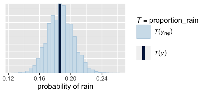

FIGURE 13.6: A posterior predictive check of the logistic regression model of rain. The histogram displays the proportion of days on which it rained in each of 100 posterior simulated datasets. The vertical line represents the observed proportion of days with rain in the weather data.

This brings us to question (3), how accurate are our posterior classifications? In the regression setting with quantitative \(Y\), we answered this question by examining the typical difference between \(Y\) and its posterior predictions. Yet in the classification setting with categorical \(Y\), our binary posterior classifications of \(Y\) are either right or wrong. What we’re interested in is how often we’re right. We will address this question in two ways: with and without cross-validation.

Let’s start by evaluating the rain_model_1 classifications of the same weather data we used to build this model. Though there’s a shortcut function in the bayesrules package, it’s important to pull back the curtain and try this by hand first. To begin, construct posterior predictive models of \(Y\) for each of the 1000 days in the weather dataset:

# Posterior predictive models for each day in dataset
set.seed(84735)
rain_pred_1 <- posterior_predict(rain_model_1, newdata = weather)
dim(rain_pred_1)
[1] 20000  1000

Each of the 1000 columns in rain_pred_1 contain 20,000 1-or-0 predictions of whether or not it will rain on the corresponding day in the weather data. As we saw in Section 13.4, each column mean indicates the proportion of these predictions that are 1 – thus the 1,000 column means estimate the probability of rain for the corresponding 1,000 days in our data. We can then convert these proportions into binary classifications of rain by comparing them to a chosen classification cut-off. We’ll start with a cut-off 0.5: if the probability of rain exceeds 0.5, then predict rain.

weather_classifications <- weather %>% 
  mutate(rain_prob = colMeans(rain_pred_1),
         rain_class_1 = as.numeric(rain_prob >= 0.5)) %>% 
  select(humidity9am, rain_prob, rain_class_1, raintomorrow)

The results for the first three days in our sample are shown below. Based on its 9 a.m. humidity level, only 12% of the 20,000 predictions called for rain on the first day (rain_prob \(=\) 0.122). Similarly, the simulated probabilities of rain for the second and third days are also amply below our 50% cut-off. As such, we predicted “no rain” for the first three sample days (as shown in rain_class_1). For the first two days, these classifications were correct – it didn’t raintomorrow. For the third day, this classification was incorrect – it did raintomorrow.

head(weather_classifications, 3)
# A tibble: 3 x 4
  humidity9am rain_prob rain_class_1 raintomorrow
        <int>     <dbl>        <dbl> <fct>       
1          55    0.122             0 No          
2          43    0.0739            0 No          
3          62    0.163             0 Yes         

Finally, to estimate our model’s overall posterior accuracy, we can compare the model classifications (rain_class_1) to the observed outcomes (raintomorrow) for each of our 1000 sample days. This information is summarized by the following table or “confusion matrix”:

# Confusion matrix
weather_classifications %>% 
  tabyl(raintomorrow, rain_class_1) %>% 
  adorn_totals(c("row", "col"))
 raintomorrow   0  1 Total
           No 803 11   814
          Yes 172 14   186
        Total 975 25  1000

Notice that our classification rule, in conjunction with our Bayesian model, correctly classified 817 of the 1000 total test cases (803 \(+\) 14). Thus, the overall classification accuracy rate is 81.7% (817 / 1000). At face value, this seems pretty good! But look closer. Our model is much better at anticipating when it won’t rain than when it will. Among the 814 days on which it doesn’t rain, we correctly classify 803, or 98.65%. This figure is referred to as the true negative rate or specificity of our Bayesian model. In stark contrast, among the 186 days on which it does rain, we correctly classify only 14, or 7.53%. This figure is referred to as the true positive rate or sensitivity of our Bayesian model. We can confirm these figures using the shortcut classification_summary() function in bayesrules:

set.seed(84735)
classification_summary(model = rain_model_1, data = weather, cutoff = 0.5)
$confusion_matrix
   y   0  1
  No 803 11
 Yes 172 14

$accuracy_rates
                        
sensitivity      0.07527
specificity      0.98649
overall_accuracy 0.81700

Sensitivity, specificity, and overall accuracy

Let \(Y\) be a set of binary response values on \(n\) data points and \(\hat{Y}\) represent the corresponding posterior classifications of \(Y\). A confusion matrix summarizes the results of these classifications relative to the actual observations where \(a + b + c + d = n\):

	\(\hat{Y} = 0\)	\(\hat{Y} = 1\)
\(Y = 0\)	\(a\)	\(b\)
\(Y = 1\)	\(c\)	\(d\)

The model’s overall accuracy captures the proportion of all \(Y\) observations that are accurately classified:

\[\text{overall accuracy} = \frac{a + d}{a + b + c + d}.\]

Further, the model’s sensitivity (true positive rate) captures the proportion of \(Y = 1\) observations that are accurately classified and specificity (true negative rate) the proportion of \(Y = 0\) observations that are accurately classified:

\[\text{sensitivity} = \frac{d}{c + d} \;\;\;\; \text{ and } \;\;\;\; \text{specificity} = \frac{a}{a + b}.\]

Now, if you fall into the reasonable group of people that don’t like walking around in wet clothes all day, the fact that our model is so bad at predicting rain is terrible news. BUT we can do better. Recall from Section 13.4 that we can adjust the classification cut-off to better suit the goals of our analysis. In our case, we can increase our model’s sensitivity by decreasing the cut-off from 0.5 to, say, 0.2. That is, we’ll classify a test case as rain if there’s even a 20% chance of rain:

set.seed(84735)
classification_summary(model = rain_model_1, data = weather, cutoff = 0.2)
$confusion_matrix
   y   0   1
  No 580 234
 Yes  67 119

$accuracy_rates
                       
sensitivity      0.6398
specificity      0.7125
overall_accuracy 0.6990

Success! By making it easier to classify rain, the sensitivity jumped from 7.53% to 63.98% (119 of 186). We’re much less likely to be walking around with wet clothes. Yet this improvement is not without consequences. In lowering the cut-off, we make it more difficult to predict when it won’t rain. As a result, the true negative rate dropped from 98.65% to 71.25% (580 of 814) and we’ll carry around an umbrella more often than we need to.

Finally, to hedge against the possibility that the above model assessments are biased by training and testing rain_model_1 using the same data, we can supplement these measures with cross-validated estimates of classification accuracy. The fact that these are so similar to our measures above suggests that the model is not overfit to our sample data – it does just as well at predicting rain on new days:⁶²

set.seed(84735)
cv_accuracy_1 <- classification_summary_cv(
  model = rain_model_1, data = weather, cutoff = 0.2, k = 10)
cv_accuracy_1$cv
  sensitivity specificity overall_accuracy
1      0.6534      0.7185            0.705

Trade-offs in sensitivity and specificity

As analysts, we must utilize context to determine an appropriate classification rule with corresponding cut-off \(c\). In doing so, there are some trade-offs to consider:

• As we lower \(c\), sensitivity increases, but specificity decreases.
• As we increase \(c\), specificity increases, but sensitivity decreases.

In closing this section, was it worth it? That is, do the benefits of better classifying rain outweigh the consequences of mistakenly classifying no rain as rain? We don’t know. This is a subjective question. As an analyst, you can continue to tweak the classification rule until the corresponding correct classification rates best match your goals.

13.6 Extending the model

As with Normal and Poisson regression models, logistic regression models can grow to accommodate more than one predictor. Recall from the introduction to this chapter that morning humidity levels at 9 a.m., \(X_{1}\), aren’t the only relevant weather observation we can make today that might help us anticipate whether or not it might rain tomorrow. We might also consider today’s afternoon humidity at 3 p.m. (\(X_2\)) and whether or not it rains today (\(X_3\)), a categorical predictor with levels No and Yes. We can plunk these predictors right into our logistic regression model:

\[\log\left(\frac{\pi_i}{1-\pi_i}\right) = \beta_0 + \beta_1 X_{i1} + \beta_2 X_{i2} + \beta_3 X_{i3} .\]

Our original prior understanding was that the chance of rain increases with each individual predictor in this model. Yet we have less prior certainty about how one predictor is related to rain when controlling for the other predictors – we’re not meteorologists or anything. For example, if we know today’s 3pm humidity level, it could very well be the case that today’s 9am humidity doesn’t add any additional information about whether or not it will rain tomorrow (i.e., \(\beta_1 = 0\)). With this, we’ll maintain our original \(N(-1.4, 0.7^2)\) prior for the centered intercept \(\beta_{0c}\), but will utilize weakly informative priors for (\(\beta_1,\beta_2,\beta_3)\):

\[\begin{split} Y_i | \beta_0, \beta_1, \beta_2, \beta_3 & \sim Bern(\pi_i) \;\; \text{ with } \;\; \log\left(\frac{\pi_i}{1-\pi_i}\right) = \beta_0 + \beta_1 X_{i1} + \beta_2 X_{i2} + \beta_3 X_{i3} \\ \beta_{0c} & \sim N(-1.4, 0.7^2) \\ \beta_1 & \sim N(0, 0.14^2) \\ \beta_2 & \sim N(0, 0.15^2) \\ \beta_3 & \sim N(0, 6.45^2). \\ \end{split}\]

We encourage you to pause here to perform a prior simulation (e.g., Do prior simulations of rain rates match our prior understanding of rain in Perth?). Here we’ll move on to simulating the corresponding posteriors for the humidity9am coefficient (\(\beta_1\)), humidity3pm coefficient (\(\beta_2\)), and raintodayYes coefficient (\(\beta_3\)) and confirm our prior specifications:

rain_model_2 <- stan_glm(
  raintomorrow ~ humidity9am + humidity3pm + raintoday, 
  data = weather, family = binomial,
  prior_intercept = normal(-1.4, 0.7),
  prior = normal(0, 2.5, autoscale = TRUE), 
  chains = 4, iter = 5000*2, seed = 84735)

# Obtain prior model specifications
prior_summary(rain_model_2)

A posterior tidy() summary is shown below. To begin, notice that the 80% credible intervals for the humidity and raintodayYes coefficients, \(\beta_2\) and \(\beta_3\), lie comfortably above 0. This suggests that, when controlling for the other predictors in the model, the chance of rain tomorrow increases with today’s 3 p.m. humidity levels and if it rained today. Looking closer, the posterior median for the raintodayYes coefficient is 1.15, equivalently \(e^{1.15} = 3.17\). Thus, when controlling for today’s morning and afternoon humidity levels, we expect that the odds of rain tomorrow more than triple if it rains today.

# Numerical summaries
tidy(rain_model_2, effects = "fixed", conf.int = TRUE, conf.level = 0.80)
# A tibble: 4 x 5
  term         estimate std.error conf.low conf.high
  <chr>           <dbl>     <dbl>    <dbl>     <dbl>
1 (Intercept)  -5.46      0.483    -6.08    -4.85   
2 humidity9am  -0.00693   0.00737  -0.0163   0.00251
3 humidity3pm   0.0796    0.00846   0.0689   0.0906 
4 raintodayYes  1.15      0.220     0.874    1.44   

In contrast, notice that the \(\beta_1\) (humidity9am) posterior straddles 0 with an 80% posterior credible interval which ranges from -0.0163 to 0.0025. Let’s start with what this observation doesn’t mean. It does not mean that humidity9am isn’t a significant predictor of tomorrow’s rain. We saw in rain_model_1 that it is. Rather, humidity9am isn’t a significant predictor of tomorrow’s rain when controlling for afternoon humidity and whether or not it rains today. Put another way, if we already know today’s humidity3pm and rain status, then knowing humidity9am doesn’t significantly improve our understanding of whether or not it rains tomorrow. This shift in understanding about humidity9am from rain_model_1 to rain_model_2 might not be much of a surprise – humidity9am is strongly associated with humidity3pm and raintoday, thus the information it holds about raintomorrow is somewhat redundant in rain_model_2.

Finally, which is the better model of tomorrow’s rain, rain_model_1 or rain_model_2? Using a classification cut-off of 0.2, let’s compare the cross-validated estimates of classification accuracy for rain_model_2 to those for rain_model_1:

set.seed(84735)
cv_accuracy_2 <- classification_summary_cv(
  model = rain_model_2, data = weather, cutoff = 0.2, k = 10)

# CV for the models
cv_accuracy_1$cv
  sensitivity specificity overall_accuracy
1      0.6534      0.7185            0.705
cv_accuracy_2$cv
  sensitivity specificity overall_accuracy
1      0.7522      0.8139            0.802

Which of rain_model_1 and rain_model_2 produces the most accurate posterior classifications of tomorrow’s rain? Which model do you prefer?

The answer to this quiz is rain_model_2. The cross-validated estimates of sensitivity, specificity, and overall accuracy jump by roughly 10 percentage points from rain_model_1 to rain_model_2. Thus, rain_model_2 is superior to rain_model_1 both in predicting when it will rain tomorrow and when it won’t. If you want even more evidence, recall from Chapter 10 that the expected log-predictive density (ELPD) measures the overall compatibility of new data points with their posterior predictive models through an examination of the log posterior predictive pdfs – the higher the ELPD the better.

# Calculate ELPD for the models
loo_1 <- loo(rain_model_1)
loo_2 <- loo(rain_model_2)

# Compare the ELPD for the 2 models
loo_compare(loo_1, loo_2)
             elpd_diff se_diff
rain_model_2   0.0       0.0  
rain_model_1 -80.2      13.5  

Here, the estimated ELPD for rain_model_1 is more than two standard errors below, and hence worse than, that of rain_model_2: (\(-80.2 \pm 2*13.5\)). Thus, ELPD provides even more evidence in favor of rain_model_2.

13.7 Chapter summary

Let response variable \(Y \in \{0,1\}\) be a binary categorical variable. Thus, modeling the relationship between \(Y\) and a set of predictors \((X_1,X_2,\ldots,X_p)\) requires a classification modeling approach. To this end, we considered the logistic regression model:

\[\begin{equation} \begin{array}{lcrl} \text{data:} & \hspace{.01in} & Y_i|\beta_0,\beta_1,\ldots,\beta_p & \stackrel{ind}{\sim} \text{Bern}(\pi_i) \;\; \text{ with } \;\; \log\left(\frac{\pi_i}{1 - \pi_i}\right) = \beta_0 + \beta_1 X_{i1} + \cdots + \beta_p X_{ip} \\ \text{priors:} & & \beta_{0c} & \sim N(m_0, s_0^2) \\ & & \beta_{1} & \sim N(m_1, s_1^2) \\ && \vdots & \\ & & \beta_{p} & \sim N(m_p, s_p^2) \\ \end{array} \tag{13.7} \end{equation}\]

where we can transform the model from the log(odds) scale to the more meaningful odds and probability scales:

\[\frac{\pi_i}{1-\pi_i} = e^{\beta_0 + \beta_1 X_{i1} + \cdots + \beta_p X_{ip}} \;\;\;\; \text{ and } \;\;\;\; \pi_i = \frac{e^{\beta_0 + \beta_1 X_{i1} + \cdots + \beta_p X_{ip}}}{1 + e^{\beta_0 + \beta_1 X_{i1} + \cdots + \beta_p X_{ip}}} .\]

While providing insight into the relationship between the outcome of \(Y\) and predictors \(X\), we can also utilize this logistic regression model to produce posterior classifications of \(Y\). In evaluating the classification quality, we must consider the overall accuracy alongside sensitivity and specificity, i.e., our model’s ability to anticipate when \(Y = 1\) and \(Y = 0\), respectively.

13.8 Exercises

13.8.1 Conceptual exercises

Exercise 13.1 (Normal vs logistic) For each scenario, identify whether Normal or logistic regression is the appropriate tool for modeling \(Y\) by \(X\).

1. \(Y\) = whether or not a person bikes to work, \(X\) = the distance from the person’s home to work
2. \(Y\) = the number of minutes it takes a person to commute to work, \(X\) = the distance from the person’s home to work
3. \(Y\) = the number of minutes it takes a person to commute to work, \(X\) = whether or not the person takes public transit to work

Exercise 13.2 (What are the odds?) Calculate and interpret the odds for each event of interest below.

1. The probability of rain tomorrow is 0.8.
2. The probability of flipping 2 Heads in a row is 0.25.
3. The log(odds) that your bus will be on time are 0.
4. The log(odds) that a person is left-handed are -1.386.

Exercise 13.3 (What’s the probability?) Calculate and interpret the probability for each event of interest below.

1. The odds that your team will win the basketball game are 20 to 1.
2. The odds of rain tomorrow are 0.5.
3. The log(odds) of a certain candidate winning the election are 1.
4. The log(odds) that a person likes pineapple pizza are -2.

Exercise 13.4 (Logistic models) Let \(Y\) indicate whether or not somebody believes that climate change is real and caused by people (TRUE or FALSE), and \(X\) be their age. The simplified posterior median logistic regression model of \(Y\) by \(X\) provides insight into the relationship between the two. NOTE: This formula is loosely based on the pulse_of_the_nation survey results in the bayesrules package.

\[\text{log(odds of belief in climate change)} = 1.43 - 0.02 \text{age}\]

1. Express the posterior median model on the odds and probability scales.
2. Interpret the age coefficient on the odds scale.
3. Calculate the posterior median probability that a 60-year-old believes in climate change.
4. Repeat part c for a 20-year-old.

Exercise 13.5 (Sensitivity vs specificity) Continuing our climate change belief analysis, the confusion matrix below summarizes the performance of our logistic model in classifying the beliefs of 1000 survey respondents, using a probability cut-off of 0.5.

y	0	1
FALSE (0)	50	300
TRUE (1)	30	620

1. Calculate and interpret the model’s overall accuracy.
2. Calculate and interpret the model’s sensitivity.
3. Calculate and interpret the model’s specificity.
4. Suppose that researchers want to improve their ability to identify people that do not believe in climate change. How might they adjust their probability cut-off: Increase it or decrease it? Why?

13.8.2 Applied exercises

Exercise 13.6 (Hotel bookings: getting started) Plans change. Hotel room bookings get canceled. In the next exercises, you’ll explore whether hotel cancellations might be predicted based upon the circumstances of a reservation. Throughout, utilize weakly informative priors and the hotel_bookings data in the bayesrules package.⁶³ Your analysis will incorporate the following variables on hotel bookings:

variable	notation	meaning
is_canceled	\(Y\)	whether or not the booking was canceled
lead_time	\(X_1\)	number of days between the booking
		and scheduled arrival
previous_cancellations	\(X_2\)	number of previous times the guest has
		canceled a booking
is_repeated_guest	\(X_3\)	whether or not the booking guest is a
		repeat customer at the hotel
average_daily_rate	\(X_4\)	the average per day cost of the hotel

1. What proportion of the sample bookings were canceled?
2. Construct and discuss plots of is_canceled vs each of the four potential predictors above.
3. Using formal mathematical notation, specify an appropriate Bayesian regression model of \(Y\) by predictors \((X_1,X_2,X_3,X_4)\).
4. Explain your choice for the structure of the data model.

Exercise 13.7 (Hotel bookings: simulation)

1. Simulate the posterior model of your regression parameters \((\beta_0,\beta_1,\ldots,\beta_4)\). Construct trace plots, density plots, and a pp_check() of the chain output.
2. Report the posterior median model of hotel cancellations on each of the log(odds), odds, and probability scales.
3. Construct 80% posterior credible intervals for your model coefficients. Interpret those for \(\beta_2\) and \(\beta_3\) on the odds scale.
4. Among the four predictors, which are significantly associated with hotel cancellations, both statistically and meaningfully? Explain.

Exercise 13.8 (Hotel bookings: classification rules)

1. How good is your model at anticipating whether a hotel booking will be canceled? Evaluate the classification accuracy using both the in-sample and cross-validation approaches, along with a 0.5 probability cut-off.
2. Are the cross-validated and in-sample assessments of classification accuracy similar? Explain why this makes sense in the context of this analysis.
3. Interpret the cross-validated overall accuracy, sensitivity, and specificity measures in the context of this analysis.
4. Thinking like a hotel booking agent, you’d like to increase the sensitivity of your classifications to 0.75. Identify a probability cut-off that you could use to achieve this level while maintaining the highest possible specificity.

Exercise 13.9 (Hotel bookings: will they cancel?!)

1. A guest that is new to a hotel and has only canceled a booking 1 time before, has booked a $100 per day hotel room 30 days in advance. Simulate, plot, and discuss the posterior predictive model of \(Y\), whether or not the guest will cancel this booking.
2. Come up with the features of another fictitious booking that’s more likely to be canceled than the booking in part a. Support your claim by simulating, plotting, and comparing this booking’s posterior predictive model of \(Y\) to that in part a.

Exercise 13.10 (Robots taking over: getting started) As engineers develop more and more sophisticated robots, there are opportunities for improved efficiency. But at what cost? Some people fear that their occupations will be replaced by robots. In the next exercises, you’ll explore whether someone’s view on robots might be associated with other survey factors. Throughout, utilize weakly informative priors and the pulse_of_the_nation survey data in the bayesrules package. Your analysis will incorporate the following variables:

variable	notation	meaning
robots	\(Y\)	0 = likely, 1 = unlikely that their jobs will be
		replaced by robots within 10 years
transformers	\(X_1\)	number of Transformers films the respondent has seen
books	\(X_2\)	number of books read in past year
age	\(X_3\)	age in years
income	\(X_4\)	income in thousands of dollars

1. What proportion of people in the sample think their job is unlikely to be taken over by robots in the next ten years?
2. Construct and discuss plots of robots vs each of the four potential predictors above.
3. Using formal mathematical notation, specify an appropriate Bayesian regression model of \(Y\) by predictors \((X_1,X_2,X_3,X_4)\).
4. Explain your choice for the structure of the data model.

Exercise 13.11 (Robots taking over: simulation)

1. Simulate the posterior model of your regression parameters \((\beta_0,\beta_1,\ldots,\beta_4)\). Construct trace plots, density plots, and a pp_check() of the chain output.
2. Report the posterior median model of a person’s robot beliefs on each of the log(odds), odds, and probability scales.
3. Construct 80% posterior credible intervals for your model coefficients. Interpret those for \(\beta_3\) and \(\beta_4\) on the odds scale.
4. Among the four predictors, which are significantly associated with thinking robots are unlikely to take over their jobs in the next 10 years, both statistically and meaningfully? Explain.

Exercise 13.12 (Robots taking over: classification rules)

1. How good is your model at anticipating whether a person is unlikely to think that their job will be taken over by a robot in the next 10 years? Evaluate the classification accuracy using both the in-sample and cross-validation approaches, along with a 0.6 probability cut-off.
2. Are the cross-validated and in-sample assessments of classification accuracy similar? Explain why this makes sense in the context of this analysis.
3. Interpret the cross-validated overall accuracy, sensitivity, and specificity measures in the context of this analysis.

13.8.3 Open-ended exercises

Exercise 13.13 (Open exercise: fake news) The fake_news data in the bayesrules package contains information about 150 news articles, some real news and some fake news. In this open-ended exercise, complete a logistic regression analysis of article type, real or fake, using the following three predictors: whether or not the article’s title includes an exclamation point (title_has_excl), the number of words in the title (title_words), and the negative sentiment rating.

Exercise 13.14 (Open exercise: ghosts are real?) We return to the pulse_of_the_nation survey data in the bayesrules package which includes a variable on whether or not a person believes in ghosts. In this open-ended exercise, complete a logistic regression analysis of whether or not someone believes in ghosts using at least three other variables from the dataset.

References

Antonio, Nuno, Ana de Almeida, and Luis Nunes. 2019. “Hotel Booking Demand Datasets.” Data in Brief 22: 41–49. https://www.sciencedirect.com/science/article/pii/S2352340918315191.

———. 2020c. “Hotels.” TidyTuesday Github Repostitory. https://github.com/rfordatascience/tidytuesday/blob/master/data/2020/2020-02-11.

---

60. Answer: d↩︎

61. weather_perth is a wrangled subset of the weatherAUS dataset in the rattle package.↩︎

62. A friendly reminder that this will be slow. We’re training, testing, and combining the results of 10 models here!↩︎

63. This is a random sample of data collected by Antonio, de Almeida, and Nunes (2019) and distributed by the Hotels TidyTuesday project (R for Data Science 2020c).↩︎