Chapter 14 Naive Bayes Classification
There exist multiple penguin species throughout Antarctica, including the Adelie, Chinstrap, and Gentoo. When encountering one of these penguins on an Antarctic trip, we might classify its species
\[Y = \begin{cases} A & \text{ Adelie} \\ C & \text{ Chinstrap} \\ G & \text{ Gentoo} \\ \end{cases}\]
by examining various physical characteristics, such as whether the penguin weighs more than the average 4200g,
\[X_{1} = \begin{cases} 1 & \text{ above-average weight} \\ 0 & \text{ below-average weight} \\ \end{cases}\]
as well as measurements of the penguin’s bill
\[\begin{split} X_{2} & = \text{ bill length (in mm)} \\ X_{3} & = \text{ flipper length (in mm)} \\ \end{split}\]
The penguins_bayes data, originally made available by Gorman, Williams, and Fraser (2014) and distributed by Horst, Hill, and Gorman (2020), contains the above species and feature information for a sample of 344 Antarctic penguins:
# Load packages
library(bayesrules)
library(tidyverse)
library(e1071)
library(janitor)

# Load data
data(penguins_bayes)
penguins <- penguins_bayes
Among these penguins, 152 are Adelies, 68 are Chinstraps, and 124 are Gentoos. We’ll assume throughout that the proportional breakdown of these species in our dataset reflects the species breakdown in the wild. That is, our prior assumption about any new penguin is that it’s most likely an Adelie and least likely a Chinstrap:
penguins %>%
  tabyl(species)
   species   n percent
    Adelie 152  0.4419
 Chinstrap  68  0.1977
    Gentoo 124  0.3605
Before proceeding with our analysis of this data, take a quick quiz.
Explain why neither the Normal nor logistic regression model would be appropriate for classifying a penguin’s species \(Y\) from its physical characteristics \(X\).
Since species \(Y\) is categorical, Normal regression isn’t an appropriate tool for understanding its relationship with physical characteristics \(X\). And though logistic regression is (currently) our only tool for modeling and classifying categorical response variables, it too is inappropriate here. Recall that with a Bernoulli data structure, the logistic regression model is limited to classifying binary response variables. Yet our species variable \(Y\) has three categories. Luckily, there’s a tool for everything. In Chapter 14 we’ll explore an alternative to logistic regression: naive Bayes classification. Relative to Bayesian logistic regression, naive Bayes classification has a few advantages:
- it can classify categorical response variables \(Y\) with two or more categories;
- it doesn’t require much theory beyond Bayes’ Rule; and
- it’s computationally efficient, i.e., doesn’t require MCMC simulation.
Sounds fantastic. But as you might expect, these benefits don’t come without a cost. We’ll observe throughout this chapter that naive Bayes classification is called “naive” for a reason.
- Explore the inner workings of naive Bayes classification.
- Implement naive Bayes classification in R.
- Develop strategies to evaluate the quality of naive Bayes classifications.
14.1 Classifying one penguin
We’ll start our naive Bayes classification with just a single penguin. Suppose an Antarctic researcher comes across a penguin that weighs less than 4200g with a 195mm-long flipper and 50mm-long bill. Our goal is to help this researcher identify the species of this penguin, Adelie, Chinstrap, or Gentoo.
14.1.1 One categorical predictor
Let’s begin by considering just the information we have on the categorical predictor \(X_1\): the penguin weighs less than 4200g, i.e., is not above_average_weight.
Take the following quiz to first build some intuition.64
Based on the plot below, for which species is a below-average weight most likely?
ggplot(penguins %>% drop_na(above_average_weight),
       aes(fill = above_average_weight, x = species)) +
  geom_bar(position = "fill")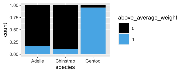
FIGURE 14.1: The proportion of each penguin species that’s above average weight.
Notice in Figure 14.1 that Chinstrap penguins are the most likely to be below average weight. Yet before declaring this penguin to be a Chinstrap, we should consider that this is the rarest species to encounter in the wild. That is, we have to think like Bayesians by combining the information from our data with our prior information about species membership to construct a posterior model for our penguin’s species. The naive Bayes classification approach to this task is nothing more than a direct appeal to the tried-and-true Bayes’ Rule from Chapter 2. In general, to calculate the posterior probability that our penguin is species \(Y = y\) in light of its weight status \(X_1 = x_1\), we can plug into
\[\begin{equation} f(y \; | \; x_1) = \frac{\text{ prior} \cdot \text{likelihood}}{\text{ normalizing constant }} = \frac{f(y)L(y \; | \; x_1)}{f(x_1)} \tag{14.1} \end{equation}\]
where, by the Law of Total Probability,
\[\begin{equation} \begin{split} f(x_1) & = \sum_{\text{all } y'} f(y')L(y' \; | \; x_1) \\ & = f(y' = A)L(y'=A|x_1) + f(y' = C)L(y'=C|x_1) + f(y' = G)L(y'=G|x_1).\\ \end{split} \tag{14.2} \end{equation}\]
A table which breaks down the above_average_weight weight status by species provides the necessary information to complete this Bayesian calculation:
penguins %>%
  select(species, above_average_weight) %>%
  na.omit() %>%
  tabyl(species, above_average_weight) %>%
  adorn_totals(c("row", "col"))
   species   0   1 Total
    Adelie 126  25   151
 Chinstrap  61   7    68
    Gentoo   6 117   123
     Total 193 149   342
In fact, we can directly calculate the posterior model of our penguin’s species from this table. For example, notice that among the 193 penguins that are below average weight, 126 are Adelies. Thus, there’s a roughly 65% posterior chance that this penguin is an Adelie:
\[f(y = A \; | \; x_1 = 0) = \frac{126}{193} \approx 0.6528 .\]
Let’s confirm this result by plugging information from our tabyl above into Bayes’ Rule (14.1).
This tedious step is not to annoy, but to practice for generalizations we’ll have to make in more complicated settings.
First, our prior information about species membership indicates that Adelies are the most common and Chinstraps the least:
\[\begin{equation} f(y = A) = \frac{151}{342}, \;\;\;\;\; f(y = C) = \frac{68}{342}, \;\;\;\;\; f(y = G) = \frac{123}{342} . \tag{14.3} \end{equation}\]
Further, the likelihoods demonstrate that below-average weight is most common among Chinstrap penguins. For example, 89.71% of Chinstraps but only 4.88% of Gentoos are below average weight:
\[\begin{split} L(y = A \; | \; x_1 = 0) & = \frac{126}{151} \approx 0.8344 \\ L(y = C \; | \; x_1 = 0) & = \frac{61}{68} \approx 0.8971 \\ L(y = G \; | \; x_1 = 0) & = \frac{6}{123} \approx 0.0488 \\ \end{split}\]
Plugging these priors and likelihoods into (14.2), the total probability of observing a below-average weight penguin across all species is
\[f(x_1 = 0) = \frac{151}{342} \cdot \frac{126}{151} + \frac{68}{342} \cdot \frac{61}{68} + \frac{123}{342} \cdot \frac{6}{123} = \frac{193}{342} .\]
Finally, by Bayes’ Rule we can confirm that there’s a 65% posterior chance that this penguin is an Adelie:
\[\begin{split} f(y = A \; | \; x_1 = 0) & = \frac{f(y = A) L(y = A \; | \; x_1 = 0)}{f(x_1 = 0)} \\ & = \frac{(151/342) \cdot (126/151)}{193/342} \\ & \approx 0.6528 . \\ \end{split}\]
Similarly, we can show that
\[f(y = C \; | \; x_1 = 0) \approx 0.3161 \;\;\;\; \text{ and } \;\;\;\; f(y = G \; | \; x_1 = 0) \approx 0.0311 . \]
All in all, the posterior probability that this penguin is an Adelie is more than double that of the other two species. Thus, our naive Bayes classification, based on our prior information and the penguin’s below-average weight alone, is that this penguin is an Adelie. Though below-average weight is relatively less common among Adelies than among Chinstraps, the final classification was pushed over the edge by the fact that Adelies are far more common.
14.1.2 One quantitative predictor
Let’s ignore the penguin’s weight for now and classify its species using only the fact that it has a 50mm-long bill. Take the following quiz to build some intuition.65
Based on Figure 14.2, among which species is a 50mm-long bill the most common?
ggplot(penguins, aes(x = bill_length_mm, fill = species)) +
  geom_density(alpha = 0.7) +
  geom_vline(xintercept = 50, linetype = "dashed")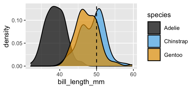
FIGURE 14.2: Density plots of the bill lengths (mm) observed among three penguin species.
Notice from the plot that a 50mm-long bill would be extremely long for an Adelie penguin. Though the distinction in bill lengths is less dramatic among the Chinstrap and Gentoo, Chinstrap bills tend to be a tad longer. In particular, a 50mm-long bill is fairly average for Chinstraps, though slightly long for Gentoos. Thus, again, our data points to our penguin being a Chinstrap. And again, we must weigh this data against the fact that Chinstraps are the rarest of these three species. To this end, we can appeal to Bayes’ Rule to make a naive Bayes classification of \(Y\) from information that bill length \(X_2 = x_2\):
\[\begin{equation} f(y \; | \; x_2) = \frac{f(y)L(y \; | \; x_2)}{f(x_2)} = \frac{f(y)L(y \; | \; x_2)}{\sum_{\text{all } y'} f(y')L(y' \; | \; x_2)} . \tag{14.4} \end{equation}\]
Our question for you is this: What is the likelihood that we would observe a 50mm-long bill if the penguin is an Adelie, \(L(y = A | x_2 = 50)\)?
Unlike the penguin’s categorical weight status (\(X_1\)), its bill length is quantitative.
Thus, we can’t simply calculate \(L(y = A \; | \; x_2 = 50)\) from a table of species vs bill_length_mm.
Further, we haven’t assumed a model for data \(X_2\) from which to define likelihood function \(L(y|x_2)\).
This is where one “naive” part of naive Bayes classification comes into play.
The naive Bayes method typically assumes that any quantitative predictor, here \(X_2\), is continuous and conditionally Normal.
That is, within each species, bill lengths \(X_2\) are Normally distributed with possibly different means \(\mu\) and standard deviations \(\sigma\):
\[\begin{split} X_2 \; | \; (Y = A) & \sim N(\mu_A, \sigma_A^2) \\ X_2 \; | \; (Y = C) & \sim N(\mu_C, \sigma_C^2) \\ X_2 \; | \; (Y = G) & \sim N(\mu_G, \sigma_G^2) \\ \end{split} .\]
Though this is a naive blanket assumption to make for all quantitative predictors, it turns out to be reasonable for bill length \(X_2\). Reexamining Figure 14.2, notice that within each species, bill lengths are roughly bell shaped around different means and with slightly different standard deviations. Thus, we can tune the Normal model for each species by setting its \(\mu\) and \(\sigma\) parameters to the observed sample means and standard deviations in bill lengths within that species. For example, we’ll tune the Normal model of bill lengths for the Adelie species to have mean and standard deviation \(\mu_A = 38.8\)mm and \(\sigma_A = 2.66\)mm:
# Calculate sample mean and sd for each Y group
penguins %>%
  group_by(species) %>%
  summarize(mean = mean(bill_length_mm, na.rm = TRUE),
            sd = sd(bill_length_mm, na.rm = TRUE))
# A tibble: 3 x 3
  species    mean    sd
  <fct>     <dbl> <dbl>
1 Adelie     38.8  2.66
2 Chinstrap  48.8  3.34
3 Gentoo     47.5  3.08
Plotting the tuned Normal models for each species confirms that this naive Bayes assumption isn’t perfect – it’s a bit more idealistic than the density plots of the raw data in Figure 14.2. But it’s fine enough to continue.
ggplot(penguins, aes(x = bill_length_mm, color = species)) +
  stat_function(fun = dnorm, args = list(mean = 38.8, sd = 2.66),
                aes(color = "Adelie")) +
  stat_function(fun = dnorm, args = list(mean = 48.8, sd = 3.34),
                aes(color = "Chinstrap")) +
  stat_function(fun = dnorm, args = list(mean = 47.5, sd = 3.08),
                aes(color = "Gentoo")) +
  geom_vline(xintercept = 50, linetype = "dashed")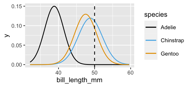
FIGURE 14.3: Normal pdfs tuned to match the observed mean and standard deviation in bill lengths (mm) among three penguin species.
Recall that this Normality assumption provides the mechanism we need to evaluate the likelihood of observing a 50mm-long bill among each of the three species, \(L(y \; | \; x_2 = 50)\).
Connecting back to Figure 14.3, these likelihoods correspond to the Normal density curve heights at a bill length of 50 mm.
Thus, observing a 50mm-long bill is slightly more likely among Chinstrap than Gentoo, and highly unlikely among Adelie penguins.
More specifically, we can calculate the likelihoods using dnorm().
# L(y = A | x_2 = 50)
dnorm(50, mean = 38.8, sd = 2.66)
[1] 2.12e-05

# L(y = C | x_2 = 50)
dnorm(50, mean = 48.8, sd = 3.34)
[1] 0.112

# L(y = G | x_2 = 50)
dnorm(50, mean = 47.5, sd = 3.08)
[1] 0.09317
We now have everything we need to plug into Bayes’ Rule (14.4). Weighting the likelihoods by the prior probabilities of each species (à la (14.2)), the marginal pdf of observing a penguin with a 50mm-long bill is
\[f(x_2 = 50) = \frac{151}{342} \cdot 0.0000212 + \frac{68}{342} \cdot 0.112 + \frac{123}{342} \cdot 0.09317 = 0.05579 .\]
Thus, the posterior probability that our penguin is an Adelie is
\[f(y = A \; | \; x_2 = 50) = \frac{(151/342) \cdot 0.0000212}{0.05579} \approx 0.0002 .\]
Similarly, we can calculate
\[f(y = C \; | \; x_2 = 50) \approx 0.3992 \;\;\;\; \text{ and } \;\;\;\; f(y = G \; | \; x_2 = 50) \approx 0.6006 . \]
It follows that our naive Bayes classification, based on our prior information and penguin’s bill length alone, is that this penguin is a Gentoo – it has the highest posterior probability. Though a 50mm-long bill is relatively less common among Gentoo than among Chinstrap, the final classification was pushed over the edge by the fact that Gentoo are much more common in the wild.
14.1.3 Two predictors
We’ve now made two naive Bayes classifications of our penguin’s species, one based solely on the fact that our penguin has below-average weight and the other based solely on its 50mm-long bill (in addition to our prior information). And these classifications disagree: we classified the penguin as Adelie in the former analysis and Gentoo in the latter. This discrepancy indicates that there’s room for improvement in our naive Bayes classification method. In particular, instead of relying on any one predictor alone, we can incorporate multiple predictors into our classification process.
Consider the information that our penguin has a bill length of \(X_2 = 50\)mm and a flipper length of \(X_3 = 195\)mm. Either one of these measurements alone might lead to a misclassification. Just as it’s tough to distinguish between the Chinstrap and Gentoo penguins based on their bill lengths alone, it’s tough to distinguish between the Chinstrap and Adelie penguins based on their flipper lengths alone (Figure 14.4).
ggplot(penguins, aes(x = bill_length_mm, fill = species)) +
  geom_density(alpha = 0.6)
ggplot(penguins, aes(x = flipper_length_mm, fill = species)) +
  geom_density(alpha = 0.6)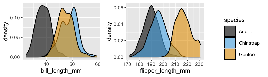
FIGURE 14.4: Density plots of the bill lengths (mm) and flipper lengths (mm) among our three penguin species.
BUT the species are fairly distinguishable when we combine the information about bill and flipper lengths. Our penguin with a 50mm-long bill and 195mm-long flipper, represented at the intersection of the dashed lines in Figure 14.5, now lies squarely among the Chinstrap observations:
ggplot(penguins,
       aes(x = flipper_length_mm, y = bill_length_mm, color = species)) +
  geom_point()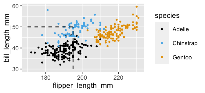
FIGURE 14.5: A scatterplot of the bill lengths (mm) versus flipper lengths (mm) among our three penguin species.
Let’s use naive Bayes classification to balance this data with our prior information on species membership. To calculate the posterior probability that the penguin is species \(Y = y\), we can adjust Bayes’ Rule to accommodate our two predictors, \(X_2 = x_2\) and \(X_3 = x_3\):
\[\begin{equation} f(y \; | \; x_2, x_3) = \frac{f(y) L(y \; | \; x_2, x_3)}{\sum_{\text{all } y'} f(y')L(y' \; | \; x_2, x_3)} . \tag{14.5} \end{equation}\]
This presents yet another new twist: How can we calculate the likelihood function that incorporates two variables, \(L(y \; | \; x_2, x_3)\)? This is where yet another “naive” assumption creeps in. Naive Bayes classification assumes that predictors are conditionally independent, thus
\[L(y \; | \; x_2, x_3) = f(x_2, x_3 \; | \; y) = f(x_2 \; | \; y)f(x_3 \; | \; y) .\]
In words, within each species, we assume that the length of a penguin’s bill has no relationship to the length of its flipper. Mathematically and computationally, this assumption makes the naive Bayes algorithm efficient and manageable. However, it might also make it wrong. Revisit Figure 14.5. Within each species, flipper length and bill length appear to be positively correlated, not independent. Yet, we’ll naively roll with the imperfect independence assumption, and thus the possibility that our classification accuracy might be weakened.
Combined then, the multivariable naive Bayes model assumes that our two predictors are Normal and conditionally independent. We already tuned this Normal model for bill length \(X_2\) in Section 14.1.2. Similarly, we can tune the species-specific Normal models for flipper length \(X_3\) to match the corresponding sample means and standard deviations:
# Calculate sample mean and sd for each Y group
penguins %>%
  group_by(species) %>%
  summarize(mean = mean(flipper_length_mm, na.rm = TRUE),
            sd = sd(flipper_length_mm, na.rm = TRUE))
# A tibble: 3 x 3
  species    mean    sd
  <fct>     <dbl> <dbl>
1 Adelie     190.  6.54
2 Chinstrap  196.  7.13
3 Gentoo     217.  6.48
Accordingly, we can evaluate the likelihood of observing a 195-mm flipper length for each of the three species, \(L(y \; | \; x_3 = 195) = f(x_3 = 195 \; | \; y)\):
# L(y = A | x_3 = 195)
dnorm(195, mean = 190, sd = 6.54)
[1] 0.04554

# L(y = C | x_3 = 195)
dnorm(195, mean = 196, sd = 7.13)
[1] 0.05541

# L(y = G | x_3 = 195)
dnorm(195, mean = 217, sd = 6.48)
[1] 0.0001934
For each species, we now have the likelihood of observing a bill length of \(X_2 = 50\) mm (Section 14.1.2), the likelihood of observing a flipper length of \(X_3 = 195\) mm (above), and the prior probability (14.3). Combined, the likelihoods of observing a 50mm-long bill and a 195mm-long flipper for each species \(Y = y\), weighted by the prior probability of the species are:
\[\begin{split} f(y' = A)L(y' = A \; | \; x_2 = 50, x_3 = 195) & = \frac{151}{342} \cdot 0.0000212 \cdot 0.04554 \\ f(y' = C)L(y' = C \; | \; x_2 = 50, x_3 = 195) & = \frac{68}{342} \cdot 0.112 \cdot 0.05541 \\ f(y' = G)L(y' = G \; | \; x_2 = 50, x_3 = 195) & = \frac{123}{342} \cdot 0.09317 \cdot 0.0001934 \\ \end{split}\]
with a sum of
\[\sum_{\text{all } y'}f(y')L(y' \; | \; x_2 = 50, x_3 = 195) \approx 0.001241 .\]
And plugging into Bayes’ Rule (14.5), the posterior probability that the penguin is an Adelie is
\[f(y = A | x_2 = 50, x_3 = 195) = \frac{\frac{151}{342} \cdot 0.0000212 \cdot 0.04554}{0.001241} \approx 0.0003 .\]
Similarly, we can calculate
\[\begin{split} f(y = C | x_2 = 50, x_3 = 195) & \approx 0.9944 \\ f(y = G | x_2 = 50, x_3 = 195) & \approx 0.0052 . \end{split}\]
In conclusion, our penguin is almost certainly a Chinstrap. Though we didn’t come to this conclusion using any physical characteristic alone, together they paint a pretty clear picture.
Naive Bayes classification
Let \(Y\) denote a categorical response variable with two or more categories and \((X_1,X_2,\dots,X_p)\) be a set of \(p\) possible predictors of \(Y\). Then the posterior probability that a new case with observed predictors \((X_1,X_2,\ldots,X_p) = (x_1,x_2,\ldots,x_p)\) belongs to class \(Y = y\) is
\[f(y | x_1, x_2, \ldots, x_p) = \frac{f(y)L(y \; | \; x_1, x_2, \ldots, x_p)}{\sum_{\text{all } y' }f(y')L(y' \; | \; x_1, x_2, \ldots, x_p)} .\]
Naive Bayes classification makes the following naive assumptions about the likelihood function of \(Y\):
Predictors \(X_i\) are conditionally independent, thus
\[L(y \; | \; x_1, x_2, \ldots, x_p) = \prod_{i=1}^p f(x_i \; | \; y)\; .\]
For categorical predictors \(X_i\), the conditional pmf
\[f(x_i \; | \; y) = P(X_i = x_i \; | \; Y = y)\]
is estimated by the sample proportion of observed \(Y = y\) cases for which \(X_i = x_i\).
For quantitative predictors \(X_i\), the conditional pmf / pdf \(f(x_i \; | \; y)\) is defined by a Normal model:
\[X_i | (Y = y) \sim N(\mu_{iy}, \sigma^2_{iy}).\]
That is, within each category \(Y = y\), we assume that \(X_i\) is Normally distributed around some mean \(\mu_{iy}\) with standard deviation \(\sigma_{iy}\). Further, we estimate \(\mu_{iy}\) and \(\sigma_{iy}\) by the sample mean and standard deviation of the observed \(X_i\) values in category \(Y = y\).
14.2 Implementing & evaluating naive Bayes classification
That was nice, but we needn’t do all of this work by hand.
To implement naive Bayes classification in R, we’ll use the naiveBayes() function in the e1071 package (Meyer et al. 2021).
As with stan_glm(), we feed naiveBayes() the data and a formula indicating which data variables to use in the analysis.
Yet, since naive Bayes calculates prior probabilities directly from the data and implementation doesn’t require MCMC simulation, we don’t have to worry about providing information regarding prior models or Markov chains.
Below we build two naive Bayes classification algorithms, one using bill_length_mm alone and one that also incorporates flipper_length_mm:
naive_model_1 <- naiveBayes(species ~ bill_length_mm, data = penguins)
naive_model_2 <- naiveBayes(species ~ bill_length_mm + flipper_length_mm,
                            data = penguins)
Let’s apply both of these to classify our_penguin that we studied throughout Section 14.1:
our_penguin <- data.frame(bill_length_mm = 50, flipper_length_mm = 195)Beginning with naive_model_1, the predict() function returns the posterior probabilities of each species along with a final classification.
This classification follows a simple rule: classify the penguin as whichever species has the highest posterior probability.
The results of this process are similar to those that we got “by hand” in Section 14.1.2, just off a smidge due to some rounding error.
Essentially, based on its bill length alone, our best guess is that this penguin is a Gentoo:
predict(naive_model_1, newdata = our_penguin, type = "raw")
       Adelie Chinstrap Gentoo
[1,] 0.000169    0.3978  0.602
predict(naive_model_1, newdata = our_penguin)
[1] Gentoo
Levels: Adelie Chinstrap Gentoo
And just as we concluded in Section 14.1.3, if we take into account both its bill length and flipper length, our best guess is that this penguin is a Chinstrap:
predict(naive_model_2, newdata = our_penguin, type = "raw")
        Adelie Chinstrap   Gentoo
[1,] 0.0003446    0.9949 0.004787
predict(naive_model_2, newdata = our_penguin)
[1] Chinstrap
Levels: Adelie Chinstrap Gentoo
We can similarly apply our naive Bayes models to classify any number of penguins. As with logistic regression, we’ll take two common approaches to evaluating the accuracy of these classifications:
- construct confusion matrices which compare the observed species of our sample penguins to their naive Bayes species classifications; and
- for a better sense of how well our naive Bayes models classify new penguins, calculate cross-validated estimates of classification accuracy.
To begin with the first approach, we classify each of the penguins using both naive_model_1 and naive_model_2 and store these in penguins as class_1 and class_2:
penguins <- penguins %>%
  mutate(class_1 = predict(naive_model_1, newdata = .),
         class_2 = predict(naive_model_2, newdata = .))
The classification results are shown below for four randomly sampled penguins, contrasted against the actual species of these penguins.
For the last two penguins, the two models produce the same classifications (Adelie) and these classifications are correct.
For the first two penguins, the two models lead to different classifications.
In both cases, naive_model_2 is correct.
set.seed(84735)
penguins %>%
  sample_n(4) %>%
  select(bill_length_mm, flipper_length_mm, species, class_1, class_2) %>%
  rename(bill = bill_length_mm, flipper = flipper_length_mm)
# A tibble: 4 x 5
   bill flipper species   class_1 class_2
  <dbl>   <int> <fct>     <fct>   <fct>
1  47.5     199 Chinstrap Gentoo  Chinstrap
2  40.9     214 Gentoo    Adelie  Gentoo
3  41.3     194 Adelie    Adelie  Adelie
4  38.5     190 Adelie    Adelie  Adelie
Of course, it remains to be seen whether naive_model_2 outperforms naive_model_1 overall.
To this end, the confusion matrices below summarize the models’ classification accuracy across all penguins in our sample.
Use these to complete the following quiz.66
- In
naive_model_1, as what other species is the Chinstrap most commonly misclassified? - Which model is better at classifying Chinstrap penguins?
- Which model has a higher overall accuracy rate?
# Confusion matrix for naive_model_1
penguins %>%
  tabyl(species, class_1) %>%
  adorn_percentages("row") %>%
  adorn_pct_formatting(digits = 2) %>%
  adorn_ns()
   species       Adelie Chinstrap       Gentoo
    Adelie 95.39% (145) 0.00% (0)  4.61%   (7)
 Chinstrap  5.88%   (4) 8.82% (6) 85.29%  (58)
    Gentoo  6.45%   (8) 4.84% (6) 88.71% (110)

# Confusion matrix for naive_model_2
penguins %>%
  tabyl(species, class_2) %>%
  adorn_percentages("row") %>%
  adorn_pct_formatting(digits = 2) %>%
  adorn_ns()
   species       Adelie   Chinstrap       Gentoo
    Adelie 96.05% (146)  2.63%  (4)  1.32%   (2)
 Chinstrap  7.35%   (5) 86.76% (59)  5.88%   (4)
    Gentoo  0.81%   (1)  0.81%  (1) 98.39% (122)
With these prompts in mind, let’s examine the two confusion matrices.
One quick observation is that naive_model_2 does a better job across the board.
Not only are its classification accuracy rates for each of the Adelie, Chinstrap, and Gentoo species higher than in naive_model_1, its overall accuracy rate is also higher.
The naive_model_2 correctly classifies 327 (146 \(+\) 59 \(+\) 122) of the 344 total penguins (95%), whereas naive_model_1 correctly classifies only 261 (76%).
Where naive_model_2 enjoys the greatest improvement over naive_model_1 is in the classification of Chinstrap penguins.
In naive_model_1, only 9% of Chinstraps are correctly classified, with a whopping 85% being misclassified as Gentoo.
At 87%, the classification accuracy rate for Chinstraps is much higher in naive_model_2.
Finally, for due diligence, we can utilize 10-fold cross-validation to evaluate and compare how well our naive Bayes classification models classify new penguins, not just those in our sample.
We do so using the naive_classification_summary_cv() function in the bayesrules package:
set.seed(84735)
cv_model_2 <- naive_classification_summary_cv(
  model = naive_model_2, data = penguins, y = "species", k = 10)
The cv_model_2$folds object contains the classification accuracy rates for each of the 10 folds whereas cv_model_2$cv averages the results across all 10 folds:
cv_model_2$cv
   species       Adelie   Chinstrap       Gentoo
    Adelie 96.05% (146)  2.63%  (4)  1.32%   (2)
 Chinstrap  7.35%   (5) 86.76% (59)  5.88%   (4)
    Gentoo  0.81%   (1)  0.81%  (1) 98.39% (122)
The accuracy rates in this cross-validated confusion matrix are comparable to those in the non-cross-validated confusion matrix above. This implies that our naive Bayes model appears to perform nearly as well on new penguins as it does on the original penguin sample that we used to build this model.
14.3 Naive Bayes vs logistic regression
Given the three penguin species categories, our classification analysis above required naive Bayes classification – taking logistic regression to this task wasn’t even an option. However, in scenarios with a binary categorical response variable \(Y\), both logistic regression and naive Bayes are viable classification approaches. In fact, we encourage you to revisit and apply naive Bayes to the rain classification example from Chapter 13. In such binary settings, the question then becomes which classification tool to use. Both naive Bayes and logistic regression have their pros and cons. Though naive Bayes is certainly computationally efficient, it also makes some very rigid and often inappropriate assumptions about data structures. You might have also noted that we lose some nuance with naive Bayes. Unlike the logistic regression model with
\[\log\left(\frac{\pi}{1 - \pi}\right) = \beta_0 + \beta_1 X_1 + \cdots + \beta_k X_p ,\]
naive Bayes lacks regression coefficients \(\beta_i\). Thus, though naive Bayes can turn information about predictors \(X\) into classifications of \(Y\), it does so without much illumination of the relationships among these variables.
Whether naive Bayes or logistic regression is the right tool for a binary classification job depends upon the situation. In general, if the rigid naive Bayes assumptions are inappropriate or if you care about the specific connections between \(Y\) and \(X\) (i.e., you don’t simply want a set of classifications), you should use logistic regression. Otherwise, naive Bayes might be just the thing. Better yet, don’t choose! Try out and learn from both tools.
14.4 Chapter summary
Naive Bayes classification is a handy tool for classifying categorical response variables \(Y\) with two or more categories. Letting \((X_1,X_2,\dots,X_p)\) be a set of \(p\) possible predictors of \(Y\), naive Bayes calculates the posterior probability of each category membership via Bayes’ Rule:
\[f(y | x_1, x_2, \ldots, x_p) = \frac{f(y)L(y \; | \; x_1, x_2, \ldots, x_p)}{\sum_{\text{all } y' }f(y')L(y' \; | \; x_1, x_2, \ldots, x_p)} .\]
In doing so, it makes some very naive assumptions about the data model from which we define the likelihood \(L(y \; | \; x_1, x_2, \ldots, x_p)\): the predictors \(X_i\) are conditionally independent and the values of quantitative predictors \(X_i\) vary Normally within each category \(Y = y\). When appropriate, these simplifying assumptions make the naive Bayes model computationally efficient and straightforward to apply. Yet when these simplifying assumptions are violated (which is common), the naive Bayes model can produce misleading classifications.
14.5 Exercises
14.5.1 Conceptual exercises
- We want to classify a person’s political affiliation \(Y\) (Democrat, Republican, or Other) by their age \(X\).
- We want to classify whether a person owns a car \(Y\) (yes or no) by their age \(X\).
- We want to classify whether a person owns a car \(Y\) (yes or no) by their location \(X\) (urban, suburban, or rural).
- Name one pro of naive Bayes classification.
- Name one con of naive Bayes classification.
14.5.2 Applied exercises
fake_news data in the bayesrules package contains information about 150 news articles, some real news and some fake news. In the next exercises, our goal will be to develop a model that helps us classify an article’s type, real or fake, using a variety of predictors. To begin, let’s consider whether an article’s title has an exclamation point (title_has_excl).
- Construct and discuss a visualization of the relationship between article
typeandtitle_has_excl. - Suppose a new article is posted online and its title does not have an exclamation point. Utilize naive Bayes classification to calculate the posterior probability that the article is real. Do so from scratch, without using
naiveBayes()withpredict(). - Check your work to part b using
naiveBayes()withpredict().
- Construct and discuss a visualization of the relationship between article
typeand the number oftitle_words. - In using naive Bayes classification to classify an article’s
typebased on itstitle_words, we assume that the number oftitle_wordsare conditionally Normal. Do you think this is a fair assumption in this analysis? - Suppose a new article is posted online and its title has 15 words. Utilize naive Bayes classification to calculate the posterior probability that the article is real. Do so from scratch, without using
naiveBayes()withpredict(). - Check your work to part c using
naiveBayes()withpredict().
title_words) and the percent of words in the article that have a negative sentiment.
- Construct and discuss a visualization of the relationship between article
typeandnegativesentiment. - Construct a visualization of the relationship of article
typewith bothtitle_wordsandnegative. - Suppose a new article is posted online – it has a 15-word title and 6% of its words have negative associations. Utilize naive Bayes classification to calculate the posterior probability that the article is real. Do so from scratch, without using
naiveBayes()withpredict(). - Check your work to part c using
naiveBayes()withpredict().
naiveBayes() with predict().
type. In this exercise you’ll evaluate and compare the performance of these four models.
| model | formula |
|---|---|
news_model_1 |
type ~ title_has_excl |
news_model_2 |
type ~ title_words |
news_model_3 |
type ~ title_words + negative |
news_model_4 |
type ~ title_words + negative + title_has_excl |
- Construct a cross-validated confusion matrix for
news_model_1. - Interpret each percentage in the confusion matrix.
- Similarly, construct cross-validated confusion matrices for the other three models.
- If our goal is to best detect when an article is fake, which of the four models should we use?
type is binary, we could also approach this task using Bayesian logistic regression.
- Starting from weakly informative priors, use
stan_glm()to simulate the posterior logistic regression model of newstypeby all three predictors:title_words,negative, andtitle_has_excl. - Perform and discuss some MCMC diagnostics.
- Construct and discuss a
pp_check(). - Using a probability cutoff of 0.5, obtain cross-validated estimates of the sensitivity and specificity for the logistic regression model.
- Compare the cross-validated metrics of the logistic regression model to those of
naive_model_4. Which model is better at detecting fake news?
14.5.3 Open-ended exercises
pulse_of_the_nation data in the bayesrules package contains responses of 1000 adults to a wide-ranging survey. In one question, respondents were asked about their belief in climate_change, selecting from the following options: climate change is Not Real at All, Real but not Caused by People, or Real and Caused by People. In this open-ended exercise, complete a naive Bayesian analysis of a person’s belief in climate_change, selecting a variety of possible predictors that are of interest to you.
pulse_of_the_nation survey also asked respondents about their agreement with the statement that vaccines_are_safe, selecting from the following options: Neither Agree nor Disagree, Somewhat Agree, Somewhat Disagree, Strongly Agree or Strongly Disagree. In this open-ended exercise, complete a naive Bayesian analysis of belief in the safety of vaccines, selecting a variety of possible predictors that are of interest to you.