Chapter 2 Bayes’ Rule
The Collins Dictionary named “fake news” the 2017 term of the year.
And for good reason.
Fake, misleading, and biased news has proliferated along with online news and social media platforms which allow users to post articles with little quality control.
It’s then increasingly important to help readers flag articles as “real” or “fake.”
In Chapter 2 you’ll explore how the Bayesian philosophy from Chapter 1 can help us make this distinction.
To this end, we’ll examine a sample of 150 articles which were posted on Facebook and fact checked by five BuzzFeed journalists (Shu et al. 2017).
Information about each article is stored in the fake_news dataset in the bayesrules package.
To learn more about this dataset, type ?fake_news in your console.
# Load packages
library(bayesrules)
library(tidyverse)
library(janitor)

# Import article data
data(fake_news)
The fake_news data contains the full text for actual news articles, both real and fake. As such, some of these articles contain disturbing language or topics. Though we believe it’s important to provide our original resources, not metadata, you do not need to read the articles in order to do the analysis ahead.
The table below, constructed using the tabyl() function in the janitor package (Firke 2021), illustrates that 40% of the articles in this particular collection are fake and 60% are real:
fake_news %>%
  tabyl(type) %>%
  adorn_totals("row")
  type   n percent
  fake  60     0.4
  real  90     0.6
 Total 150     1.0
Using this information alone, we could build a very simple news filter which uses the following rule: since most articles are real, we should read and believe all articles. This filter would certainly solve the problem of mistakenly disregarding real articles, but at the cost of reading lots of fake news. It also only takes into account the overall rates of, not the typical features of, real and fake news. For example, suppose that the most recent article posted to a social media platform is titled: “The president has a funny secret!” Some features of this title probably set off some red flags. For example, the usage of an exclamation point might seem like an odd choice for a real news article. Our data backs up this instinct – in our article collection, 26.67% (16 of 60) of fake news titles but only 2.22% (2 of 90) of real news titles use an exclamation point:
# Tabulate exclamation usage and article type
fake_news %>%
  tabyl(title_has_excl, type) %>%
  adorn_totals("row")
 title_has_excl fake real
          FALSE   44   88
           TRUE   16    2
          Total   60   90
Thus, we have two pieces of contradictory information. Our prior information suggested that incoming articles are most likely real. However, the exclamation point data is more consistent with fake news. Thinking like Bayesians, we know that balancing both pieces of information is important in developing a posterior understanding of whether the article is fake (Figure 2.1).
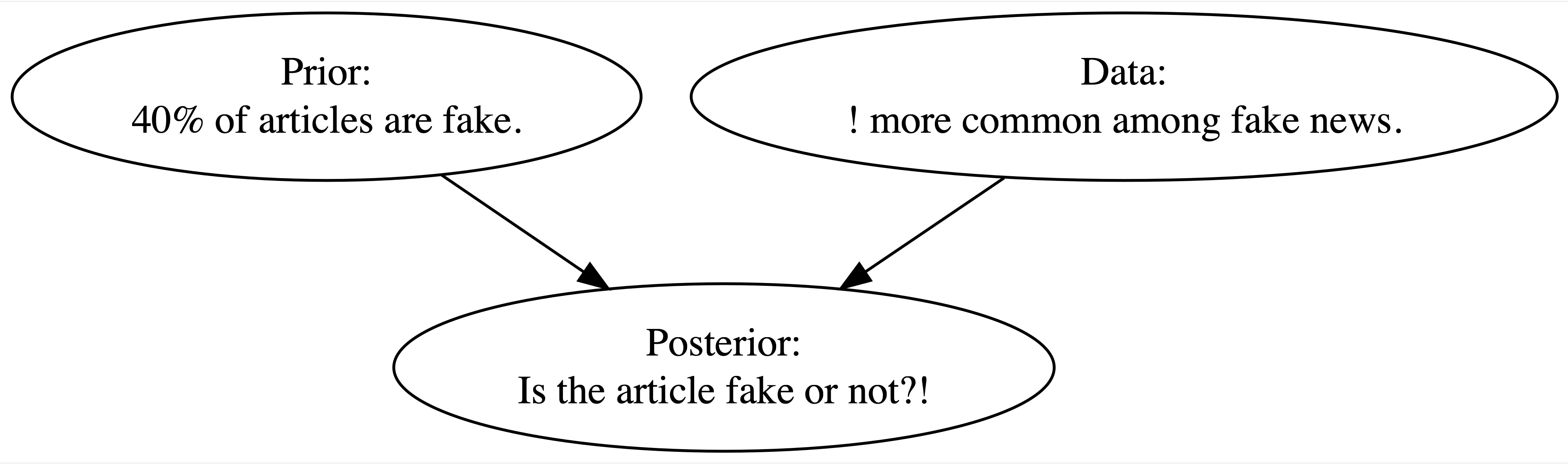
FIGURE 2.1: Bayesian knowledge-building diagram for whether or not the article is fake.
Put your own Bayesian thinking to use in a quick self-quiz of your current intuition about whether the most recent article is fake.
What best describes your updated, posterior understanding about the article?
- The chance that this article is fake drops from 40% to 20%. The exclamation point in the title might simply reflect the author’s enthusiasm.
- The chance that this article is fake jumps from 40% to roughly 90%. Though exclamation points are more common among fake articles, let’s not forget that only 40% of articles are fake.
- The chance that this article is fake jumps from 40% to roughly 98%. Given that so few real articles use exclamation points, this article is most certainly fake.
The correct answer is given in the footnote below.11 But if your intuition was incorrect, don’t fret. By the end of Chapter 2, you will have learned how to support Bayesian thinking with rigorous Bayesian calculations using Bayes’ Rule, the aptly named foundation of Bayesian statistics. And heads up: of any other chapter in this book, Chapter 2 introduces the most Bayesian concepts, notation, and vocabulary. No matter your level of previous probability experience, you’ll want to take this chapter slowly. Further, our treatment focuses on the probability tools that are necessary to Bayesian analyses. For a broader probability introduction, we recommend that the interested reader visit Chapters 1 through 3 and Section 7.1 of Blitzstein and Hwang (2019).
Explore foundational probability tools such as marginal, conditional, and joint probability models and the Binomial model.
Conduct your first formal Bayesian analysis! You will construct your first prior and data models and, from these, construct your first posterior models via Bayes’ Rule.
Practice your Bayesian grammar. Imagnie how dif ficult it would beto reed this bok if the authers didnt spellcheck or use proper grammar and! punctuation. In this spirit, you’ll practice the formal notation and terminology central to Bayesian grammar.
Simulate Bayesian models. Simulation is integral to building intuition for and supporting Bayesian analyses. You’ll conduct your first simulation, using the R statistical software, in this chapter.
2.1 Building a Bayesian model for events
Our fake news analysis boils down to the study of two variables: an article’s fake vs real status and its use of exclamation points. These features can vary from article to article. Some are fake, some aren’t. Some use exclamation points, some don’t. We can represent the randomness in these variables using probability models. In this section we will build a prior probability model for our prior understanding of whether the most recent article is fake; a model for interpreting the exclamation point data; and, eventually, a posterior probability model which summarizes the posterior plausibility that the article is fake.
2.1.1 Prior probability model
As a first step in our Bayesian analysis, we’ll formalize our prior understanding of whether the new article is fake.
Based on our fake_news data, which we’ll assume is a fairly representative sample, we determined earlier that 40% of articles are fake and 60% are real.
That is, before even reading the new article, there’s a 0.4 prior probability that it’s fake and a 0.6 prior probability it’s not.
We can represent this information using mathematical notation.
Letting \(B\) denote the event that an article is fake and \(B^c\) (read “\(B\) complement” or “B not”) denote the event that it’s not fake, we have
\[P(B) = 0.40 \;\; \text{ and } \;\; P(B^c) = 0.60 .\]
As a collection, \(P(B)\) and \(P(B^c)\) specify the simple prior model of fake news in Table 2.1. As a valid probability model must: (1) it accounts for all possible events (all articles must be fake or real); (2) it assigns prior probabilities to each event; and (3) these probabilities sum to one.
| event | \(B\) | \(B^c\) | Total |
|---|---|---|---|
| probability | 0.4 | 0.6 | 1 |
2.1.2 Conditional probability & likelihood
In the second step of our Bayesian analysis, we’ll summarize the insights from the data we collected on the new article. Specifically, we’ll formalize our observation that the exclamation point data is more compatible with fake news than with real news. Recall that if an article is fake, then there’s a roughly 26.67% chance it uses exclamation points in the title. In contrast, if an article is real, then there’s only a roughly 2.22% chance it uses exclamation points. When stated this way, it’s clear that the occurrence of exclamation points depends upon, or is conditioned upon, whether the article is fake. This dependence is specified by the following conditional probabilities of exclamation point usage (\(A\)) given an article’s fake status (\(B\) or \(B^c\)):
\[P(A | B) = 0.2667 \;\; \text{ and } \;\; P(A | B^c) = 0.0222.\]
Conditional vs unconditional probability
Let \(A\) and \(B\) be two events. The unconditional probability of \(A\), \(P(A)\), measures the probability of observing \(A\), without any knowledge of \(B\). In contrast, the conditional probability of \(A\) given \(B\), \(P(A|B)\), measures the probability of observing \(A\) in light of the information that \(B\) occurred.
Conditional probabilities are fundamental to Bayesian analyses, and thus a quick pause to absorb this concept is worth it. In general, comparing the conditional vs unconditional probabilities, \(P(A|B)\) vs \(P(A)\), reveals the extent to which information about \(B\) informs our understanding of \(A\). In some cases, the certainty of an event \(A\) might increase in light of new data \(B\). For example, if somebody practices the clarinet every day, then their probability of joining an orchestra’s clarinet section is higher than that among the general population12:
\[P(\text{orchestra} \; | \; \text{practice}) > P(\text{orchestra}) .\]
Conversely, the certainty of an event might decrease in light of new data. For example, if you’re a fastidious hand washer, then you’re less likely to get the flu:
\[P(\text{flu} \; | \; \text{wash hands}) < P(\text{flu}) .\]
The order of conditioning is also important. Since they measure two different phenomena, it’s typically the case that \(P(A|B) \ne P(B|A)\). For instance, roughly 100% of puppies are adorable. Thus, if the next object you pass on the street is a puppy, \(P(\text{adorable} \; | \; \text{puppy}) = 1\). However, the reverse is not true. Not every adorable object is a puppy, thus \(P(\text{puppy} \; | \; \text{adorable}) < 1\).
Finally, information about \(B\) doesn’t always change our understanding of \(A\). For example, suppose your friend has a yellow pair of shoes and a blue pair of shoes, thus four shoes in total. They choose a shoe at random and don’t show it to you. Without actually seeing the shoe, there’s a 0.5 probability that it goes on the right foot: \(P(\text{right foot}) = 2/4\). And even if they tell you that they happened to get one of the two yellow shoes, there’s still a 0.5 probability that it goes on the right foot: \(P(\text{right foot} \; | \; \text{yellow}) = 1/2\). That is, information about the shoe’s color tells us nothing about which foot it fits – shoe color and foot are independent.
Independent events
Two events \(A\) and \(B\) are independent if and only if the occurrence of \(B\) doesn’t tell us anything about the occurrence of \(A\):
\[P(A|B) = P(A) .\]
Let’s reexamine our fake news example with these conditional concepts in place. The conditional probabilities we derived above, \(P(A | B) =\) 0.2667 and \(P(A | B^c) =\) 0.0222, indicate that a whopping 26.67% of fake articles versus a mere 2.22% of real articles use exclamation points. Since exclamation point usage is so much more likely among fake news than real news, this data provides some evidence that the article is fake. We should congratulate ourselves on this observation – we’ve evaluated the exclamation point data by flipping the conditional probabilities \(P(A|B)\) and \(P(A|B^c)\) on their heads. For example, on its face, the conditional probability \(P(A|B)\) measures the uncertainty in event \(A\) given we know event \(B\) occurs. However, we find ourselves in the opposite situation. We know that the incoming article used exclamation points, \(A\). What we don’t know is whether or not the article is fake, \(B\) or \(B^c\). Thus, in this case, we compared \(P(A|B)\) and \(P(A|B^c)\) to ascertain the relative likelihoods of observing data \(A\) under different scenarios of the uncertain article status. To help distinguish this application of conditional probability calculations from that when \(A\) is uncertain and \(B\) is known, we’ll utilize the following likelihood function notation \(L(\cdot | A)\):
\[L(B|A) = P(A|B) \;\; \text{ and } \;\; L(B^c|A) = P(A|B^c).\]
We present a general definition below, but be patient with yourself here. The distinction is subtle, especially since people use the terms “likelihood” and “probability” interchangeably in casual conversation.
Probability vs likelihood
When \(B\) is known, the conditional probability function \(P(\cdot | B)\) allows us to compare the probabilities of an unknown event, \(A\) or \(A^c\), occurring with \(B\):
\[P(A|B) \; \text{ vs } \; P(A^c|B).\]
When \(A\) is known, the likelihood function \(L( \cdot | A) = P(A | \cdot)\) allows us to evaluate the relative compatibility of data \(A\) with events \(B\) or \(B^c\):
\[L(B|A) \; \text{ vs } \; L(B^c|A).\]
Table 2.2 summarizes the information that we’ve amassed thus far, including the prior probabilities and likelihoods associated with the new article being fake or real, \(B\) or \(B^c\). Notice that the prior probabilities add up to 1 but the likelihoods do not. Again, the likelihood function is not a probability function, but rather provides a framework to compare the relative compatibility of our exclamation point data with \(B\) and \(B^c\). Thus, whereas the prior evidence suggested the article is most likely real (\(P(B) < P(B^c)\)), the data is more consistent with the article being fake (\(L(B|A) > L(B^c|A)\)).
| event | \(B\) | \(B^c\) | Total |
|---|---|---|---|
| prior probability | 0.4 | 0.6 | 1 |
| likelihood | 0.2667 | 0.0222 | 0.2889 |
2.1.3 Normalizing constants
Though the likelihood function in Table 2.2 nicely summarizes exclamation point usage in real vs fake news, the marginal probability of observing exclamation points across all news articles, \(P(A)\), provides an important point of comparison. In our quest to calculate this normalizing constant,13 we’ll first use our prior model and likelihood function to fill in the table below. This table summarizes the possible joint occurrences of the fake news and exclamation point variables. We encourage you to take a crack at this before reading on, utilizing the information we’ve gathered on exclamation points.
| \(B\) | \(B^c\) | Total | |
|---|---|---|---|
| \(A\) | |||
| \(A^c\) | |||
| Total | 0.4 | 0.6 | 1 |
First, focus on the \(B\) column which splits fake articles into two groups: (1) those that are fake and use exclamation points, denoted \(A \cap B\); and (2) those that are fake and don’t use exclamation points, denoted \(A^c \cap B\).14 To determine the probabilities of these joint events, note that 40% of articles are fake and 26.67% of fake articles use exclamation points, \(P(B) =\) 0.4 and \(P(A|B) =\) 0.2667. It follows that across all articles, 26.67% of 40%, or 10.67%, are fake with exclamation points. That is, the joint probability of observing both \(A\) and \(B\) is
\[P(A \cap B) = P(A|B)P(B) = 0.2667 \cdot 0.4 = 0.1067.\]
Further, since 26.67% of fake articles use exclamation points, 73.33% do not. That is, the conditional probability that an article does not use exclamation points (\(A^c\)) given it’s fake (\(B\)) is:
\[P(A^c|B) = 1 - P(A|B) = 1 - 0.2667 = 0.7333.\]
It follows that 73.33% of 40%, or 29.33%, of all articles are fake without exclamation points:
\[P(A^c \cap B) = P(A^c|B)P(B) = 0.7333 \cdot 0.4 = 0.2933 .\]
In summary, the total probability of observing a fake article is the sum of its parts:
\[P(B) = P(A \cap B) + P(A^c \cap B) = 0.1067 + 0.2933 = 0.4 .\]
We can similarly break down real articles into those that do and those that don’t use exclamation points. Across all articles, only 1.33% (2.22% of 60%) are real and use exclamation points whereas 58.67% (97.78% of 60%) are real without exclamation points:
\[\begin{split} P(A \cap B^c) & = P(A|B^c)P(B^c) = 0.0222 \cdot 0.6 = 0.0133 \\ P(A^c \cap B^c) & = P(A^c|B^c)P(B^c) = 0.9778 \cdot 0.6 = 0.5867.\\ \end{split}\]
Thus, the total probability of observing a real article is the sum of these two parts:
\[P(B^c) = P(A \cap B^c) + P(A^c \cap B^c) = 0.0133 + 0.5867 = 0.6 .\]
In these calculations, we intuited a general formula for calculating joint probabilities \(P(A \cap B)\) and, through rearranging, a formula for conditional probabilities \(P(A|B)\).
Calculating joint and conditional probabilities
For events \(A\) and \(B\), the joint probability of \(A \cap B\) is calculated by weighting the conditional probability of \(A\) given \(B\) by the marginal probability of \(B\):
\[\begin{equation} P(A \cap B) = P(A | B)P(B). \tag{2.1} \end{equation}\]
Thus, when \(A\) and \(B\) are independent,
\[P(A \cap B) = P(A)P(B).\]
Dividing both sides of (2.1) by \(P(B)\), and assuming \(P(B) \ne 0\), reveals the definition of the conditional probability of \(A\) given \(B\):
\[\begin{equation} P(A | B) = \frac{P(A \cap B)}{P(B)}. \tag{2.2} \end{equation}\]
Thus, to evaluate the chance that \(A\) occurs in light of information \(B\), we can consider the chance that they occur together, \(P(A \cap B)\), relative to the chance that \(B\) occurs at all, \(P(B)\).
Table 2.3 summarizes our new understanding of the joint behavior of our two article variables. The fact that the grand total of this table is one confirms that our calculations are reasonable. Table 2.3 also provides the point of comparison we sought: 12% of all news articles use exclamation points, \(P(A) =\) 0.12. So that we needn’t always build similar marginal probabilities from scratch, let’s consider the theory behind this calculation. As usual, we can start by recognizing the two ways that an article can use exclamation points: if it is fake (\(A \cap B\)) and if it is not fake (\(A \cap B^c\)). Thus, the total probability of observing \(A\) is the combined probability of these distinct parts:
\[P(A) = P(A \cap B) + P(A \cap B^c).\]
By (2.1), we can compute the two pieces of this puzzle using the information we have about exclamation point usage among fake and real news, \(P(A|B)\) and \(P(A|B^c)\), weighted by the prior probabilities of fake and real news, \(P(B)\) and \(P(B^c)\):
\[\begin{equation} \begin{split} P(A) & = P(A \cap B) + P(A \cap B^c) = P(A|B)P(B) + P(A|B^c)P(B^c) . \end{split} \tag{2.3} \end{equation}\]
Finally, plugging in, we can confirm that roughly 12% of all articles use exclamation points: \(P(A) = 0.2667 \cdot 0.4 + 0.0222 \cdot 0.6 = 0.12\). The formula we’ve built to calculate \(P(A)\) here is a special case of the aptly named Law of Total Probability (LTP).
| \(B\) | \(B^c\) | Total | |
|---|---|---|---|
| \(A\) | 0.1067 | 0.0133 | 0.12 |
| \(A^c\) | 0.2933 | 0.5867 | 0.88 |
| Total | 0.4 | 0.6 | 1 |
2.1.4 Posterior probability model via Bayes’ Rule!
We’re now in a position to answer the ultimate question: What’s the probability that the latest article is fake? Formally speaking, we aim to calculate the posterior probability that the article is fake given that it uses exclamation points, \(P(B|A)\). To build some intuition, let’s revisit Table 2.3. Since our article uses exclamation points, we can zoom in on the 12% of articles that fall into the \(A\) row. Among these articles, proportionally 88.9% (0.1067 / 0.12) are fake and 11.1% (0.0133 / 0.12) are real. Though it might feel anti-climactic, this is the answer we were seeking: there’s an 88.9% posterior chance that this latest article is fake.
Stepping back from the details, we’ve accomplished something big: we built Bayes’ Rule from scratch! In short, Bayes’ Rule provides the mechanism we need to put our Bayesian thinking into practice. It defines a posterior model for an event \(B\) from two pieces: the prior probability of \(B\) and the likelihood of observing data \(A\) if \(B\) were to occur.
Bayes’ Rule for events
For events \(A\) and \(B\), the posterior probability of \(B\) given \(A\) follows by combining (2.2) with (2.1) and recognizing that we can evaluate data \(A\) through the likelihood function, \(L(B|A) = P(A|B)\) and \(L(B^c|A) = P(A|B^c)\):
\[\begin{equation} P(B |A) = \frac{P(A \cap B)}{P(A)} = \frac{P(B)L(B|A)}{P(A)} \tag{2.4} \end{equation}\]
where by the Law of Total Probability (2.3)
\[\begin{equation} P(A) = P(B)L(B|A) + P(B^c)L(B^c|A) . \tag{2.5} \end{equation}\]
More generally,
\[\text{posterior} = \frac{\text{prior } \cdot \text{ likelihood}}{\text{normalizing constant}} .\]
To convince ourselves that Bayes’ Rule works, let’s directly apply it to our news analysis. Into (2.4), we can plug the prior information that 40% of articles are fake, the 26.67% likelihood that a fake article would use exclamation points, and the 12% marginal probability of observing exclamation points across all articles. The resulting posterior probability that the incoming article is fake is roughly 0.889, just as we calculated from Table 2.3:
\[P(B|A) = \frac{P(B)L(B|A)}{P(A)} = \frac{ 0.4 \cdot 0.2667}{0.12} = 0.889 .\]
Table 2.4 summarizes our news analysis journey, from the prior to the posterior model. We started with a prior understanding that there’s only a 40% chance that the incoming article would be fake. Yet upon observing the use of an exclamation point in the title “The president has a funny secret!”, a feature that’s more common to fake news, our posterior understanding evolved quite a bit – the chance that the article is fake jumped to 88.9%.
| event | \(B\) | \(B^c\) | Total |
|---|---|---|---|
| prior probability | 0.4 | 0.6 | 1 |
| posterior probability | 0.889 | 0.111 | 1 |
2.1.5 Posterior simulation
It’s important to keep in mind that the probability models we built for our news analysis above are just that – models.
They provide theoretical representations of what we observe in practice.
To build intuition for the connection between the articles that might actually be posted to social media and their underlying models, let’s run a simulation.
First, define the possible article type, real or fake, and their corresponding prior probabilities:
# Define possible articles
article <- data.frame(type = c("real", "fake"))

# Define the prior model
prior <- c(0.6, 0.4)
To simulate the articles that might be posted to your social media, we can use the sample_n() function in the dplyr package (Wickham et al. 2021) to randomly sample rows from the article data frame.
In doing so, we must specify the sample size and that the sample should be taken with replacement (replace = TRUE).
Sampling with replacement ensures that we start with a fresh set of possibilities for each article – any article can either be fake or real.
Finally, we set weight = prior to specify that there’s a 60% chance an article is real and a 40% chance it’s fake.
To try this out, run the following code multiple times, each time simulating three articles.
# Simulate 3 articles
sample_n(article, size = 3, weight = prior, replace = TRUE)
Notice that you can get different results every time you run this code.
That’s because simulation, like articles, is random.
Specifically, behind the R curtain is a random number generator (RNG) that’s in charge of producing random samples.
Every time we ask for a new sample, the RNG “starts” at a new place: the random seed.
Starting at different seeds can thus produce different samples.
This is a great thing in general – random samples should be random.
However, within a single analysis, we want to be able to reproduce our random simulation results, i.e., we don’t want the fine points of our results to change every time we re-run our code.
To achieve this reproducibility, we can specify or set the seed by applying the set.seed() function to a positive integer (here 84735).
Run the below code a few times and notice that the results are always the same – the first two articles are fake and the third is real:15
# Set the seed. Simulate 3 articles.
set.seed(84735)
sample_n(article, size = 3, weight = prior, replace = TRUE)
  type
1 fake
2 fake
3 real
We’ll use set.seed() throughout the book so that readers can reproduce and follow our work. But it’s important to remember that these results are still random. Reflecting the potential error and variability in simulation, different seeds would typically give different numerical results though similar conclusions.
Now that we understand how to simulate a few articles, let’s dream bigger: simulate 10,000 articles and store the results in article_sim.
# Simulate 10000 articles.
set.seed(84735)
article_sim <- sample_n(article, size = 10000,
                        weight = prior, replace = TRUE)
The composition of the 10,000 simulated articles is summarized by the bar plot below, constructed using the ggplot() function in the ggplot2 package (Wickham 2016):
ggplot(article_sim, aes(x = type)) +
  geom_bar()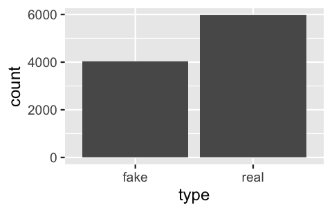
FIGURE 2.2: A bar plot of the fake vs real status of 10,000 simulated articles.
The table below provides a more thorough summary. Reflecting the model from which these 10,000 articles were generated, roughly (but not exactly) 40% are fake:
article_sim %>%
  tabyl(type) %>%
  adorn_totals("row")
  type     n percent
  fake  4031  0.4031
  real  5969  0.5969
 Total 10000  1.0000
Next, let’s simulate the exclamation point usage among these 10,000 articles.
The data_model variable specifies that there’s a 26.67% chance that any fake article and a 2.22% chance that any real article uses exclamation points:
article_sim <- article_sim %>%
  mutate(data_model = case_when(type == "fake" ~ 0.2667,
                                type == "real" ~ 0.0222))

glimpse(article_sim)
Rows: 10,000
Columns: 2
$ type       <chr> "fake", "fake", "real", "fake", "f…
$ data_model <dbl> 0.2667, 0.2667, 0.0222, 0.2667, 0.…
From this data_model, we can simulate whether each article includes an exclamation point.
This syntax is a bit more complicated.
First, the group_by() statement specifies that the exclamation point simulation is to be performed separately for each of the 10,000 articles.
Second, we use sample() to simulate the exclamation point data, no or yes, based on the data_model and store the results as usage.
Note that sample() is similar to sample_n() but samples values from vectors instead of rows from data frames.
# Define whether there are exclamation points
data <- c("no", "yes")

# Simulate exclamation point usage
set.seed(3)
article_sim <- article_sim %>%
  group_by(1:n()) %>%
  mutate(usage = sample(data, size = 1,
                        prob = c(1 - data_model, data_model)))
The article_sim data frame now contains 10,000 simulated articles with different features, summarized in the table below.
The patterns here reflect the underlying likelihoods that roughly 28% (1070 / 4031) of fake articles and 2% (136 / 5969) of real articles use exclamation points.
article_sim %>%
  tabyl(usage, type) %>%
  adorn_totals(c("col","row"))
 usage fake real Total
    no 2961 5833  8794
   yes 1070  136  1206
 Total 4031 5969 10000
Figure 2.3 provides a visual summary of these article characteristics. Whereas the left plot reflects the relative breakdown of exclamation point usage among real and fake news, the right plot frames this information within the normalizing context that only roughly 12% (1206 / 10000) of all articles use exclamation points.
ggplot(article_sim, aes(x = type, fill = usage)) +
  geom_bar(position = "fill")
ggplot(article_sim, aes(x = type)) +
  geom_bar()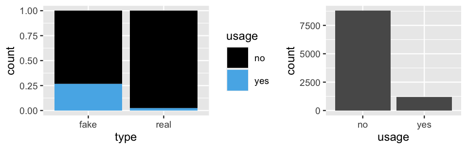
FIGURE 2.3: Bar plots of exclamation point usage, both within fake vs real news and overall.
Our 10,000 simulated articles now reflect the prior model of fake news, as well as the likelihood of exclamation point usage among fake vs real news. In turn, we can use them to approximate the posterior probability that the latest article is fake. To this end, we can filter out the simulated articles that match our data (i.e., those that use exclamation points) and examine the percentage of articles that are fake:
article_sim %>%
  filter(usage == "yes") %>%
  tabyl(type) %>%
  adorn_totals("row")
  type    n percent
  fake 1070  0.8872
  real  136  0.1128
 Total 1206  1.0000
Among the 1206 simulated articles that use exclamation points, roughly \(88.7\)% are fake. This approximation is quite close to the actual posterior probability of 0.889. Of course, our posterior assessment of this article would change if we had seen different data, i.e., if the title didn’t have exclamation points. Figure 2.4 reveals a simple rule: If an article uses exclamation points, it’s most likely fake. Otherwise, it’s most likely real (and we should read it!). NOTE: The same rule does not apply to this real book in which the liberal use of exclamation points simply conveys our enthusiasm!
ggplot(article_sim, aes(x = type)) +
  geom_bar() +
  facet_wrap(~ usage)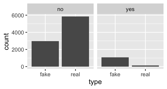
FIGURE 2.4: Bar plots of real vs fake news, broken down by exclamation point usage.
2.2 Example: Pop vs soda vs coke
Let’s put Bayes’ Rule into action in another example. Our word choices can reflect where we live. For example, suppose you’re watching an interview of somebody that lives in the United States. Without knowing anything about this person, U.S. Census figures provide prior information about the region in which they might live: the Midwest (\(M\)), Northeast (\(N\)), South (\(S\)), or West (\(W\)).16 This prior model is summarized in Table 2.5.17 Notice that the South is the most populous region and the Northeast the least (\(P(S) > P(N)\)). Thus, based on population statistics alone, there’s a 38% prior probability that the interviewee lives in the South:
\[P(S) = 0.38 .\]
| region | M | N | S | W | Total |
|---|---|---|---|---|---|
| probability | 0.21 | 0.17 | 0.38 | 0.24 | 1 |
But then, you see the person point to a fizzy cola drink and say “please pass my pop.”
Though the country is united in its love of fizzy drinks, it’s divided in what they’re called, with common regional terms including “pop,” “soda,” and “coke.”
This data, i.e., the person’s use of “pop,” provides further information about where they might live.
To evaluate this data, we can examine the pop_vs_soda dataset in the bayesrules package (Dogucu, Johnson, and Ott 2021) which includes 374250 responses to a volunteer survey conducted at popvssoda.com.
To learn more about this dataset, type ?pop_vs_soda in your console.
Though the survey participants aren’t directly representative of the regional populations (Table 2.5), we can use their responses to approximate the likelihood of people using the word pop in each region:
# Load the data
data(pop_vs_soda)

# Summarize pop use by region
pop_vs_soda %>%
  tabyl(pop, region) %>%
  adorn_percentages("col")
   pop midwest northeast   south   west
 FALSE  0.3553    0.7266 0.92078 0.7057
  TRUE  0.6447    0.2734 0.07922 0.2943
Letting \(A\) denote the event that a person uses the word “pop,” we’ll thus assume the following regional likelihoods:
\[L(M|A) = 0.6447, \;\;\;\; L(N|A) = 0.2734, \;\;\;\; L(S|A) = 0.0792, \;\;\;\; L(W|A) = 0.2943\]
For example, 64.47% of people in the Midwest but only 7.92% of people in the South use the term “pop.” Comparatively then, the “pop” data is most likely if the interviewee lives in the Midwest and least likely if they live in the South, with the West and Northeast being in between these two extremes: \(L(M|A) > L(W|A) > L(N|A) > L(S|A)\).
Weighing the prior information about regional populations with the data that the interviewee used the word “pop,” what are we to think now? For example, considering the fact that 38% of people live in the South but that “pop” is relatively rare to that region, what’s the posterior probability that the interviewee lives in the South? Per Bayes’ Rule (2.4), we can calculate this probability by
\[\begin{equation} P(S | A) = \frac{P(S)L(S|A)}{P(A)} . \tag{2.6} \end{equation}\]
We already have two of the three necessary pieces of the puzzle, the prior probability \(P(S)\) and likelihood \(L(S|A)\). Consider the third, the marginal probability that a person uses the term “pop” across the entire U.S., \(P(A)\). By extending the Law of Total Probability (2.5), we can calculate \(P(A)\) by combining the likelihoods of using “pop” in each region, while accounting for the regional populations. Accordingly, there’s a 28.26% chance that a person in the U.S. uses the word “pop”:
\[\begin{split} P(A) & = L(M|A)P(M) + L(N|A)P(N) + L(S|A)P(S) + L(W|A)P(W) \\ & = 0.6447 \cdot 0.21 + 0.2734 \cdot 0.17 + 0.0792 \cdot 0.38 + 0.2943 \cdot 0.24\\ & \approx 0.2826 . \\ \end{split}\]
Then plugging into (2.6), there’s a roughly 10.65% posterior chance that the interviewee lives in the South:
\[P(S | A) = \frac{0.38 \cdot 0.0792}{0.2826}\; \approx 0.1065 .\] We can similarly update our understanding of the interviewee living in the Midwest, Northeast, or West. Table 2.6 summarizes the resulting posterior model of region alongside the original prior. Soak it in. Upon hearing the interviewee use “pop,” we now think it’s most likely that they live in the Midwest and least likely that they live in the South, despite the South being the most populous region.
| region | M | N | S | W | Total |
|---|---|---|---|---|---|
| prior probability | 0.21 | 0.17 | 0.38 | 0.24 | 1 |
| posterior probability | 0.4791 | 0.1645 | 0.1065 | 0.2499 | 1 |
2.3 Building a Bayesian model for random variables
In our Bayesian analyses above, we constructed posterior models for categorical variables. In the fake news analysis, we examined the categorical status of an article: fake or real. In the pop vs soda example, we examined the categorical outcome of an interviewee’s region: Midwest, Northeast, South, or West. However, it’s often the case in a Bayesian analysis that our outcomes of interest are numerical. Though some of the details will change, the same Bayes’ Rule principles we built above generalize to the study of numerical random variables.
2.3.1 Prior probability model
In 1996, world chess champion (and human!) Gary Kasparov played a much anticipated six-game chess match against the IBM supercomputer Deep Blue. Of the six games, Kasparov won three, drew two, and lost one. Thus, Kasparov won the overall match, preserving the notion that machines don’t perform as well as humans when it comes to chess. Yet Kasparov and Deep Blue were to meet again for a six-game match in 1997. Let \(\pi\), read “pi” or “pie,” denote Kasparov’s chances of winning any particular game in the re-match.18 Thus, \(\pi\) is a measure of his overall skill relative to Deep Blue. Given the complexity of chess, machines, and humans, \(\pi\) is unknown and can vary or fluctuate over time. Or, in short, \(\pi\) is a random variable.
As with the fake news analysis, our analysis of random variable \(\pi\) will start with a prior model which (1) identifies what values \(\pi\) can take, and (2) assigns a prior weight or probability to each, where (3) these probabilities sum to 1. Consider the prior model defined in Table 2.7. We’ll get into how we might build such a prior in later chapters. For now, let’s focus on interpreting and utilizing the given prior.
| \(\pi\) | 0.2 | 0.5 | 0.8 | Total |
|---|---|---|---|---|
| \(f(\pi)\) | 0.10 | 0.25 | 0.65 | 1 |
The first thing you might notice is that this model greatly simplifies reality.19 Though Kasparov’s win probability \(\pi\) can technically be any number from zero to one, this prior assumes that \(\pi\) has a discrete set of possibilities: Kasparov’s win probability is either 20%, 50%, or 80%. Next, examine the probability mass function (pmf) \(f(\cdot)\) which specifies the prior probability of each possible \(\pi\) value. This pmf reflects the prior understanding that Kasparov learned from the 1996 match-up, and so will most likely improve in 1997. Specifically, this pmf places a 65% chance on Kasparov’s win probability jumping to \(\pi = 0.8\) and only a 10% chance on his win probability dropping to \(\pi = 0.2\), i.e., \(f(\pi = 0.8) = 0.65\) and \(f(\pi = 0.2) = 0.10\).
Discrete probability model
Let \(Y\) be a discrete random variable. The probability model of \(Y\) is specified by a probability mass function (pmf) \(f(y)\). This pmf defines the probability of any given outcome \(y\),
\[f(y) = P(Y = y)\]
and has the following properties:
- \(0 \le f(y) \le 1\) for all \(y\); and
- \(\sum_{\text{all } y} f(y) = 1\), i.e., the probabilities of all possible outcomes \(y\) sum to 1.
2.3.2 The Binomial data model
In the second step of our Bayesian analysis, we’ll collect and process data which can inform our understanding of \(\pi\), Kasparov’s skill level relative to that of Deep Blue. Here, our data \(Y\) is the number of the six games in the 1997 re-match that Kasparov wins.20 Since the chess match outcome isn’t predetermined, \(Y\) is a random variable that can take any value in \(\{0,1,...,6\}\). Further, \(Y\) inherently depends upon Kasparov’s win probability \(\pi\). If \(\pi\) were 0.80, Kasparov’s victories \(Y\) would also tend to be high. If \(\pi\) were 0.20, \(Y\) would tend to be low. For our formal Bayesian analysis, we must model this dependence of \(Y\) on \(\pi\). That is, we must develop a conditional probability model of how \(Y\) depends upon or is conditioned upon the value of \(\pi\).
Conditional probability model of data \(Y\)
Let \(Y\) be a discrete random variable and \(\pi\) be a parameter upon which \(Y\) depends. Then the conditional probability model of \(Y\) given \(\pi\) is specified by conditional pmf \(f(y|\pi)\). This pmf specifies the conditional probability of observing \(y\) given \(\pi\),
\[f(y|\pi) = P(Y = y | \pi)\]
and has the following properties:
- \(0 \le f(y|\pi) \le 1\) for all \(y\); and
- \(\sum_{\text{all } y} f(y|\pi) = 1\).
In modeling the dependence of \(Y\) on \(\pi\) in our chess example, we first make two assumptions about the chess match: (1) the outcome of any one game doesn’t influence the outcome of another, i.e., games are independent; and (2) Kasparov has an equal probability, \(\pi\), of winning any game in the match, i.e., his chances don’t increase or decrease as the match goes on. This is a common framework in statistical analysis, one which can be represented by the Binomial model.
The Binomial model
Let random variable \(Y\) be the number of successes in a fixed number of trials \(n\). Assume that the trials are independent and that the probability of success in each trial is \(\pi\). Then the conditional dependence of \(Y\) on \(\pi\) can be modeled by the Binomial model with parameters \(n\) and \(\pi\). In mathematical notation:
\[Y | \pi \sim \text{Bin}(n,\pi) \]
where “\(\sim\)” can be read as “modeled by.” Correspondingly, the Binomial model is specified by conditional pmf
\[\begin{equation} f(y|\pi) = \left(\!\begin{array}{c} n \\ y \end{array}\!\right) \pi^y (1-\pi)^{n-y} \;\; \text{ for } y \in \{0,1,2,\ldots,n\} \tag{2.7} \end{equation}\]
where \(\left(\!\begin{array}{c} n \\ y \end{array}\!\right) = \frac{n!}{y!(n-y)!}\).
We can now say that the dependence of Kasparov’s victories \(Y\) in \(n = 6\) games on his win probability \(\pi\) follows a Binomial model,
\[Y | \pi \sim \text{Bin}(6,\pi)\]
with conditional pmf
\[\begin{equation} f(y|\pi) = \left(\!\begin{array}{c} 6 \\ y \end{array}\!\right) \pi^y (1 - \pi)^{6 - y} \;\; \text{ for } y \in \{0,1,2,3,4,5,6\} . \tag{2.8} \end{equation}\]
This pmf summarizes the conditional probability of observing any number of wins \(Y = y\) for any given win probability \(\pi\). For example, if Kasparov’s underlying chance of beating Deep Blue were \(\pi = 0.8\), then there’s a roughly 26% chance he’d win all six games:
\[f(y = 6 | \pi = 0.8) = \left(\!\begin{array}{c} 6 \\ 6 \end{array}\!\right) 0.8^6 (1 - 0.8)^{6 - 6} = 1 \cdot 0.8^6 \cdot 1 \approx 0.26 .\]
And a near 0 chance he’d lose all six games:
\[f(y = 0 | \pi = 0.8) = \left(\!\begin{array}{c} 6 \\ 0 \end{array}\!\right) 0.8^0 (1 - 0.8)^{6 - 0} = 1 \cdot 1 \cdot 0.2^6 \approx 0.000064 .\]
Figure 2.5 plots the conditional pmfs \(f(y|\pi)\), and thus the random outcomes of \(Y\), under each possible value of Kasparov’s win probability \(\pi\). These plots confirm our intuition that Kasparov’s victories \(Y\) would tend to be low if Kasparov’s win probability \(\pi\) were low (far left) and high if \(\pi\) were high (far right).
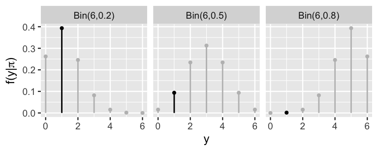
FIGURE 2.5: The pmf of a Bin(6, \(\pi\)) model is plotted for each possible value of \(\pi \in \{0.2, 0.5, 0.8\}\). The masses marked by the black lines correspond to the eventual observed data, \(Y = 1\) win.
2.3.3 The Binomial likelihood function
The Binomial provides a theoretical model of the data \(Y\) we might observe. In the end, Kasparov only won one of the six games against Deep Blue in 1997 (\(Y = 1\)). Thus, the next step in our Bayesian analysis is to determine how compatible this particular data is with the various possible \(\pi\). Put another way, we want to evaluate the likelihood of Kasparov winning \(Y = 1\) game under each possible \(\pi\). It turns out that the answer is staring us straight in the face. Extracting only the masses in Figure 2.5 that correspond to our observed data, \(Y = 1\), reveals the likelihood function of \(\pi\) (Figure 2.6).
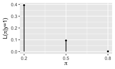
FIGURE 2.6: The likelihood function \(L(\pi|y = 1)\) of observing \(Y = 1\) win in six games for any win probability \(\pi \in \{0.2, 0.5, 0.8\}\).
Just as the likelihood in our fake news example was obtained by flipping a conditional probability on its head, the formula for the likelihood function follows from evaluating the conditional pmf \(f(y|\pi)\) in (2.8) at the observed data \(Y = 1\). For \(\pi \in \{0.2,0.5,0.8\}\),
\[L(\pi | y = 1) = f(y=1 | \pi) = \left(\!\begin{array}{c} 6 \\ 1 \end{array}\!\right) \pi^1 (1-\pi)^{6-1} = 6\pi(1-\pi)^5 . \]
Table 2.8 summarizes the likelihood function evaluated at each possible value of \(\pi\). For example, there’s a low 0.0015 likelihood of Kasparov winning just one game if he were the superior player, i.e., \(\pi = 0.8\):
\[L(\pi = 0.8 | y = 1) = 6\cdot 0.8 \cdot (1-0.8)^5 \approx 0.0015 . \]
There are some not-to-miss details here. First, though it is equivalent in formula to the conditional pmf of \(Y\), \(f(y=1 | \pi)\), we use the \(L(\pi | y = 1)\) notation to reiterate that the likelihood is a function of the unknown win probability \(\pi\) given the observed \(Y = 1\) win data. In fact, the resulting likelihood formula depends only upon \(\pi\). Further, the likelihood function does not sum to one across \(\pi\), and thus is not a probability model. (Mental gymnastics!) Rather, it provides a mechanism by which to compare the compatibility of the observed data \(Y = 1\) with different \(\pi\).
| \(\pi\) | 0.2 | 0.5 | 0.8 |
|---|---|---|---|
| \(L(\pi | y=1)\) | 0.3932 | 0.0938 | 0.0015 |
Putting this all together, the likelihood function summarized in Figure 2.6 and Table 2.8 illustrates that Kasparov’s one game win is most consistent with him being the weaker player and least consistent with him being the better player: \(L(\pi = 0.2 | y = 1) > L(\pi = 0.5 | y = 1) > L(\pi = 0.8 | y = 1)\). In fact, it’s nearly impossible that Kasparov would have only won one game if his win probability against Deep Blue were as high as \(\pi = 0.8\): \(L(\pi = 0.8 | y = 1) \approx 0\).
Probability mass functions vs likelihood functions
When \(\pi\) is known, the conditional pmf \(f(\cdot | \pi)\) allows us to compare the probabilities of different possible values of data \(Y\) (e.g., \(y_1\) or \(y_2\)) occurring with \(\pi\):
\[f(y_1|\pi) \; \text{ vs } \; f(y_2|\pi) .\]
When \(Y=y\) is known, the likelihood function \(L(\cdot | y) = f(y | \cdot)\) allows us to compare the relative likelihood of observing data \(y\) under different possible values of \(\pi\) (e.g., \(\pi_1\) or \(\pi_2\)):
\[L(\pi_1|y) \; \text{ vs } \; L(\pi_2|y) .\]
Thus, \(L(\cdot | y)\) provides the tool we need to evaluate the relative compatibility of data \(Y=y\) with various \(\pi\) values.
2.3.4 Normalizing constant
Consider where we are. In contrast to our prior model of \(\pi\) (Table 2.7), our 1997 chess match data provides evidence that Deep Blue is now the dominant player (Table 2.8). As Bayesians, we want to balance this prior and likelihood information. Our mechanism for doing so, Bayes’ Rule, requires three pieces of information: the prior, likelihood, and a normalizing constant. We’ve taken care of the first two, now let’s consider the third. To this end, we must determine the total probability that Kasparov would win \(Y = 1\) game across all possible win probabilities \(\pi\), \(f(y = 1)\). As we did in our other examples, we can appeal to the Law of Total Probability (LTP) to calculate \(f(y = 1)\). The idea is this. The overall probability of Kasparov’s one win outcome (\(Y = 1\)) is the sum of its parts: the likelihood of observing \(Y = 1\) with a win probability \(\pi\) that’s either 0.2, 0.5, or 0.8 weighted by the prior probabilities of these \(\pi\) values. Taking a little leap from the LTP for events (2.5), this means that
\[f(y = 1) = \sum_{\pi \in \{0.2,0.5,0.8\}} L(\pi | y=1) f(\pi)\]
or, expanding the summation \(\Sigma\) and plugging in the prior probabilities and likelihoods from Tables 2.7 and 2.8:
\[\begin{equation} \begin{split} f(y = 1) & = L(\pi = 0.2 | y=1) f(\pi = 0.2) + L(\pi = 0.5 | y=1) f(\pi = 0.5) \\ & \hspace{.2in} + L(\pi = 0.8 | y=1) f(\pi = 0.8) \\ & \approx 0.3932 \cdot 0.10 + 0.0938 \cdot 0.25 + 0.0015 \cdot 0.65 \\ & \approx 0.0637 . \\ \end{split} \tag{2.9} \end{equation}\]
Thus, across all possible \(\pi\), there’s only a roughly 6% chance that Kasparov would have won only one game. It would, of course, be great if this all clicked. But if it doesn’t, don’t let this calculation discourage you from moving forward. We’ll learn a magical shortcut in Section 2.3.6 that allows us to bypass this calculation.
2.3.5 Posterior probability model
Figure 2.7 summarizes what we know thus far and where we have yet to go. Heading into their 1997 re-match, our prior model suggested that Kasparov’s win probability against Deep Blue was high (left plot). But! Then he only won one of six games, a result that is most likely when Kasparov’s win probability is low (middle plot). Our updated, posterior model (right plot) of Kasparov’s win probability will balance this prior and likelihood. Specifically, our formal calculations below will verify that Kasparov’s chances of beating Deep Blue most likely dipped to \(\pi = 0.20\) between 1996 to 1997. It’s also relatively possible that his 1997 losing streak was a fluke, and that he’s more evenly matched with Deep Blue (\(\pi = 0.50\)). In contrast, it’s highly unlikely that Kasparov is still the superior player (\(\pi = 0.80\)).
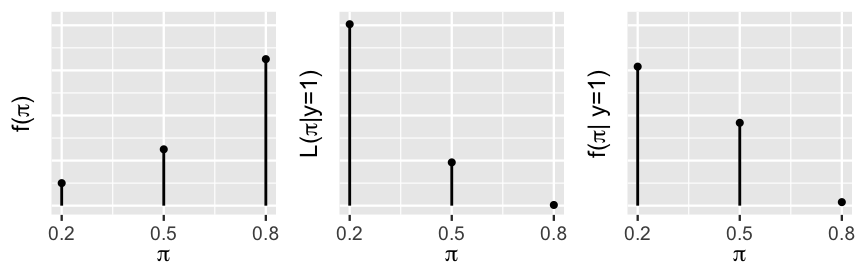
FIGURE 2.7: The prior (left), likelihood (middle), and posterior (right) models of \(\pi\). The y-axis scales are omitted for ease of comparison.
The posterior model plotted in Figure 2.7 is specified by the posterior pmf
\[f(\pi | y = 1) .\]
Conceptually, \(f(\pi | y=1)\) is the posterior probability of some win probability \(\pi\) given that Kasparov only won one of six games against Deep Blue. Thus, defining the posterior \(f(\pi | y = 1)\) isn’t much different than it was in our previous examples. Just as you might hope, Bayes’ Rule still holds:
\[\text{ posterior } = \; \frac{\text{ prior } \cdot \text{ likelihood }}{\text{normalizing constant}} .\]
In the chess setting, we can translate this as
\[\begin{equation} f(\pi | y=1) = \frac{f(\pi)L(\pi|y=1)}{f(y = 1)} \;\; \text{ for } \pi \in \{0.2,0.5,0.8\} . \tag{2.10} \end{equation}\]
All that remains is a little “plug-and-chug”: the prior \(f(\pi)\) is defined by Table 2.7, the likelihood \(L(\pi|y=1)\) by Table 2.8, and the normalizing constant \(f(y=1)\) by (2.9). The posterior probabilities follow:
\[\begin{equation} \begin{split} f(\pi = 0.2 | y = 1) & = \frac{0.10 \cdot 0.3932}{0.0637} \approx 0.617 \\ f(\pi = 0.5 | y = 1) & = \frac{0.25 \cdot 0.0938}{0.0637} \approx 0.368 \\ f(\pi = 0.8 | y = 1) & = \frac{0.65 \cdot 0.0015}{0.0637} \approx 0.015 \\ \end{split} \tag{2.11} \end{equation}\]
This posterior probability model is summarized in Table 2.9 along with the prior probability model for comparison. These details confirm the trends in and intuition behind Figure 2.7. Mainly, though we were fairly confident that Kasparov’s performance would have improved from 1996 to 1997, after winning only one game, the chances of Kasparov being the dominant player (\(\pi = 0.8\)) dropped from 0.65 to 0.015. In fact, the scenario with the greatest posterior support is that Kasparov is the weaker player, with a win probability of only 0.2. Good news for machines. Bad news for humans.
| \(\pi\) | 0.2 | 0.5 | 0.8 | Total |
|---|---|---|---|---|
| \(f(\pi)\) | 0.10 | 0.25 | 0.65 | 1 |
| \(f(\pi | y=1)\) | 0.617 | 0.368 | 0.015 | 1 |
We close this section by generalizing the tools we built for the chess analysis.
Bayes’ Rule for variables
For any variables \(\pi\) and \(Y\), let \(f(\pi)\) denote the prior pmf of \(\pi\) and \(L(\pi|y)\) denote the likelihood function of \(\pi\) given observed data \(Y=y\). Then the posterior pmf of \(\pi\) given data \(Y=y\) is
\[\begin{equation} f(\pi | y) = \frac{\text{ prior } \cdot \text{ likelihood }}{\text{ normalizing constant }} = \frac{f(\pi)L(\pi|y)}{f(y)} \tag{2.12} \end{equation}\]
where, by the Law of Total Probability, the overall probability of observing data \(Y=y\) across all possible \(\pi\) is
\[\begin{equation} f(y) = \sum_{\text{all } \pi} f(\pi)L(\pi|y). \tag{2.13} \end{equation}\]
2.3.6 Posterior shortcut
We now make good on our promise that, moving forward, we needn’t continue calculating the normalizing constant. To begin, notice in (2.11) that \(f(y = 1) = 0.0637\) appears in the denominator of \(f(\pi|y=1)\) for each \(\pi \in \{0.2,0.5,0.8\}\). This explains the term normalizing constant – its only purpose is to normalize the posterior probabilities so that they sum to one:
\[f(\pi = 0.2 | y = 1) + f(\pi = 0.5 | y = 1) + f(\pi = 0.8 | y = 1) = 1 . \]
Yet we needn’t actually calculate \(f(y=1)\) to normalize the posterior probabilities. Instead, we can simply note that \(f(y=1)\) is some constant \(1/c\), and thus replace (2.11) with
\[\begin{split} f(\pi = 0.2 | y = 1) & = c \cdot 0.10 \cdot 0.3932 \propto 0.039320 \\ f(\pi = 0.5 | y = 1) & = c \cdot 0.25 \cdot 0.0938 \propto 0.023450 \\ f(\pi = 0.8 | y = 1) & = c \cdot 0.65 \cdot 0.0015 \propto 0.000975 \\ \end{split}\]
where \(\propto\) denotes “proportional to.” Though these unnormalized posterior probabilities don’t add up to one,
\[0.039320 + 0.023450 + 0.000975 = 0.063745,\]
Figure 2.8 demonstrates that they preserve the proportional relationships of the normalized posterior probabilities.
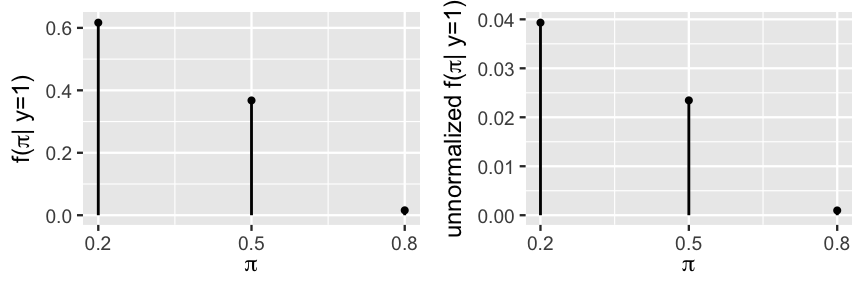
FIGURE 2.8: The normalized posterior pmf of \(\pi\) (left) and the unnormalized posterior pmf of \(\pi\) (right) with different y-axis scales.
Thus, to normalize these unnormalized probabilities while preserving their relative relationships, we can compare each to the whole. Specifically, we can divide each unnormalized probability by their sum. For example:
\[f(\pi = 0.2 | y = 1) = \frac{0.039320}{0.039320 + 0.023450 + 0.000975} \approx 0.617 .\]
Though we’ve just intuited this result, it also follows mathematically by combining (2.12) and (2.13):
\[f(\pi | y) = \frac{f(\pi)L(\pi|y)}{f(y)} = \frac{f(\pi)L(\pi|y)}{\sum_{\text{all } \pi} f(\pi)L(\pi|y)} .\]
We state the general form of this proportionality result below and will get plenty of practice with this concept in the coming chapters.
Proportionality
Since \(f(y)\) is merely a normalizing constant which does not depend on \(\pi\), the posterior pmf \(f(\pi|y)\) is proportional to the product of \(f(\pi)\) and \(L(\pi|y)\):
\[f(\pi | y) = \frac{f(\pi)L(\pi|y)}{f(y)} \propto f(\pi)L(\pi|y) .\]
That is,
\[\text{ posterior } \propto \text{ prior } \cdot \text{ likelihood }.\]
The significance of this proportionality is that all the information we need to build the posterior model is held in the prior and likelihood.
2.3.7 Posterior simulation
We’ll conclude this section with a simulation that provides insight into and supports our Bayesian analysis of Kasparov’s chess skills. Ultimately, we’ll simulate 10,000 scenarios of the six-game chess series. To begin, set up the possible values of win probability \(\pi\) and the corresponding prior model \(f(\pi)\):
# Define possible win probabilities
chess <- data.frame(pi = c(0.2, 0.5, 0.8))

# Define the prior model
prior <- c(0.10, 0.25, 0.65)
Next, simulate 10,000 possible outcomes of \(\pi\) from the prior model and store the results in the chess_sim data frame.
# Simulate 10000 values of pi from the prior
set.seed(84735)
chess_sim <- sample_n(chess, size = 10000, weight = prior, replace = TRUE)
From each of the 10,000 prior plausible values pi, we can simulate six games and record Kasparov’s number of wins, y. Since the dependence of y on pi follows a Binomial model, we can directly simulate y using the rbinom() function with size = 6 and prob = pi.
# Simulate 10000 match outcomes
chess_sim <- chess_sim %>%
  mutate(y = rbinom(10000, size = 6, prob = pi))

# Check it out
chess_sim %>%
  head(3)
   pi y
1 0.5 3
2 0.5 3
3 0.8 4
The combined 10,000 simulated pi values closely approximate the prior model \(f(\pi)\) (Table 2.7):
# Summarize the prior
chess_sim %>%
  tabyl(pi) %>%
  adorn_totals("row")
    pi     n percent
   0.2  1017  0.1017
   0.5  2521  0.2521
   0.8  6462  0.6462
 Total 10000  1.0000
Further, the 10,000 simulated match outcomes y illuminate the dependence of these outcomes on Kasparov’s win probability pi, closely mimicking the conditional pmfs \(f(y|\pi)\) from Figure 2.5.
# Plot y by pi
ggplot(chess_sim, aes(x = y)) +
  stat_count(aes(y = ..prop..)) +
  facet_wrap(~ pi)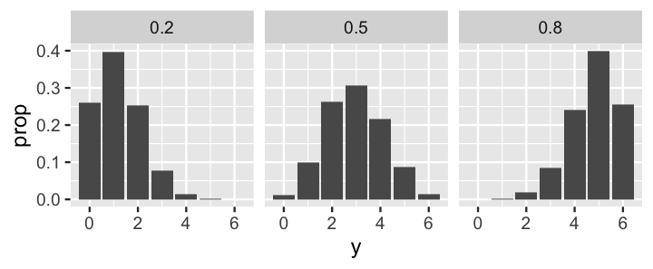
FIGURE 2.9: A bar plot of simulated win outcomes \(y\) under each possible win probability \(\pi\).
Finally, let’s focus on the simulated outcomes that match the observed data that Kasparov won one game. Among these simulations, the majority (60.4%) correspond to the scenario in which Kasparov’s win probability \(\pi\) was 0.2 and very few (1.8%) correspond to the scenario in which \(\pi\) was 0.8. These observations very closely approximate the posterior model of \(\pi\) which we formally built above (Table 2.9).
# Focus on simulations with y = 1
win_one <- chess_sim %>%
  filter(y == 1)

# Summarize the posterior approximation
win_one %>%
  tabyl(pi) %>%
  adorn_totals("row")
    pi   n percent
   0.2 404 0.60389
   0.5 253 0.37818
   0.8  12 0.01794
 Total 669 1.00000

# Plot the posterior approximation
ggplot(win_one, aes(x = pi)) +
  geom_bar()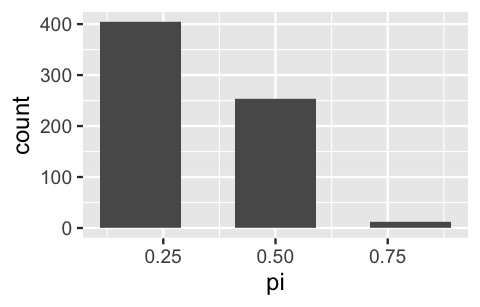
FIGURE 2.10: A bar plot of 10,000 simulated \(\pi\) values which approximates the posterior model.
2.4 Chapter summary
In Chapter 2, you learned Bayes’ Rule and that Bayes Rules! Every Bayesian analysis consists of four common steps.
Construct a prior model for your variable of interest, \(\pi\). The prior model specifies two important pieces of information: the possible values of \(\pi\) and the relative prior plausibility of each.
Summarize the dependence of data \(Y\) on \(\pi\) via a conditional pmf \(f(y|\pi)\).
Upon observing data \(Y = y\), define the likelihood function \(L(\pi|y) = f(y|\pi)\) which encodes the relative likelihood of observing data \(Y = y\) under different \(\pi\) values.
Build the posterior model of \(\pi\) via Bayes’ Rule which balances the prior and likelihood:
\[\begin{equation*} \text{posterior} = \frac{\text{prior} \cdot \text{likelihood}}{\text{normalizing constant}} \propto \text{prior} \cdot \text{likelihood}. \end{equation*}\]
More technically,
\[f(\pi|y) = \frac{f(\pi)L(\pi|y)}{f(y)} \propto f(\pi)L(\pi|y).\]
2.5 Exercises
2.5.1 Building up to Bayes’ Rule
- \(A\) = you just finished reading Lambda Literary Award-winning author Nicole Dennis-Benn’s first novel, and you enjoyed it! \(B\) = you will also enjoy Benn’s newest novel.
- \(A\) = it’s 0 degrees Fahrenheit in Minnesota on a January day. \(B\) = it will be 60 degrees tomorrow.
- \(A\) = the authors only got 3 hours of sleep last night. \(B\) = the authors make several typos in their writing today.
- \(A\) = your friend includes three hashtags in their tweet. \(B\) = the tweet gets retweeted.
- 73% of people that drive 10 miles per hour above the speed limit get a speeding ticket.
- 20% of residents drive 10 miles per hour above the speed limit.
- 15% of residents have used R.
- 91% of statistics students at the local college have used R.
- 38% of residents are Minnesotans that like the music of Prince.
- 95% of the Minnesotan residents like the music of Prince.
- At a certain hospital, an average of 6 babies are born each hour. Let \(Y\) be the number of babies born between 9 a.m. and 10 a.m. tomorrow.
- Tulips planted in fall have a 90% chance of blooming in spring. You plant 27 tulips this year. Let \(Y\) be the number that bloom.
- Each time they try out for the television show Ru Paul’s Drag Race, Alaska has a 17% probability of succeeding. Let \(Y\) be the number of times Alaska has to try out until they’re successful.
- \(Y\) is the amount of time that Henry is late to your lunch date.
- \(Y\) is the probability that your friends will throw you a surprise birthday party even though you said you hate being the center of attention and just want to go out to eat.
- You invite 60 people to your “\(\pi\) day” party, none of whom know each other, and each of whom has an 80% chance of showing up. Let \(Y\) be the total number of guests at your party.
2.5.2 Practice Bayes’ Rule for events
- What’s the prior probability that the selected tree has mold?
- The tree happens to be a maple. What’s the probability that the employee would have selected a maple?
- What’s the posterior probability that the selected maple tree has mold?
- Compare the prior and posterior probability of the tree having mold. How did your understanding change in light of the fact that the tree is a maple?
- What’s the probability that a randomly chosen person on this dating app is non-binary?
- Given that Matt is looking at the profile of someone who is non-binary, what’s the posterior probability that he swipes right?
- Mine is on a morning flight. What’s the probability that her flight will be delayed?
- Alicia’s flight is not delayed. What’s the probability that she’s on a morning flight?
| good mood | bad mood | total | |
|---|---|---|---|
| 0 texts | |||
| 1-45 texts | |||
| 46+ texts | |||
| Total | 1 |
- Use the provided information to fill in the table above.
- Today’s a new day. Without knowing anything about the previous day’s text messages, what’s the probability that your roommate is in a good mood? What part of the Bayes’ Rule equation is this: the prior, likelihood, normalizing constant, or posterior?
- You surreptitiously took a peek at your roommate’s phone (we are attempting to withhold judgment of this dastardly maneuver) and see that your roommate received 50 text messages yesterday. How likely are they to have received this many texts if they’re in a good mood today? What part of the Bayes’ Rule equation is this?
- What is the posterior probability that your roommate is in a good mood given that they received 50 text messages yesterday?
- What’s the probability they identify as LGBTQ?
- If they identify as LGBTQ, what’s the probability that they live in a rural area?
- If they do not identify as LGBTQ, what’s the probability that they live in a rural area?
2.5.3 Practice Bayes’ Rule for random variables
| \(\pi\) | 0.3 | 0.4 | 0.5 | Total |
|---|---|---|---|---|
| \(f(\pi)\) | 0.25 | 0.60 | 0.15 | 1 |
- Let \(Y\) be the number of internship offers that Muhammad gets. Specify the model for the dependence of \(Y\) on \(\pi\) and the corresponding pmf, \(f(y|\pi)\).
- Muhammad got some pretty amazing news. He was offered four of the six internships! How likely would this be if \(\pi = 0.3\)?
- Construct the posterior model of \(\pi\) in light of Muhammad’s internship news.
| \(\pi\) | 0.1 | 0.25 | 0.4 | Total |
|---|---|---|---|---|
| \(f(\pi)\) | 0.2 | 0.45 | 0.35 | 1 |
- Miles has enough clay for 7 handles. Let \(Y\) be the number of handles that will be good enough for a mug. Specify the model for the dependence of \(Y\) on \(\pi\) and the corresponding pmf, \(f(y|\pi)\).
- Miles pulls 7 handles and only 1 of them is good enough for a mug. What is the posterior pmf of \(\pi\), \(f(\pi|y=1)\)?
- Compare the posterior model to the prior model of \(\pi\). How would you characterize the differences between them?
- Miles’ instructor Kris had a different prior for his ability to pull a handle (below). Find Kris’s posterior \(f(\pi|y=1)\) and compare it to Miles’.
\(\pi\) 0.1 0.25 0.4 Total \(f(\pi)\) 0.15 0.15 0.7 1
| \(\pi\) | 0.4 | 0.5 | 0.6 | 0.7 | Total |
|---|---|---|---|---|---|
| \(f(\pi)\) | 0.1 | 0.2 | 0.44 | 0.26 | 1 |
- Fatima surveys a random sample of 80 adults and 47 are lactose intolerant. Without doing any math, make a guess at the posterior model of \(\pi\), and explain your reasoning.
- Calculate the posterior model. How does this compare to your guess in part a?
- If Fatima had instead collected a sample of 800 adults and 470 (keeping the sample proportion the same as above) are lactose intolerant, how does that change the posterior model?
- Convert the information from the 20 surveyed commuters into a prior model for \(\pi\).
- Li Qiang wants to update that prior model with the data she collected: in 13 days, the 8:30am bus was late 3 times. Find the posterior model for \(\pi\).
- Compare and comment on the prior and posterior models. What did Li Qiang learn about the bus?
| \(\pi\) | 0.6 | 0.65 | 0.7 | 0.75 | Total |
|---|---|---|---|---|---|
| \(f(\pi)\) | 0.3 | 0.4 | 0.2 | 0.1 | 1 |
- If the previous researcher had been more sure that a hatchling would survive, how would the prior model be different?
- If the previous researcher had been less sure that a hatchling would survive, how would the prior model be different?
- Lisa collects some data. Among the 15 hatchlings she studied, 10 survived for at least one week. What is the posterior model for \(\pi\)?
- Lisa needs to explain the posterior model for \(\pi\) in a research paper for ornithologists, and can’t assume they understand Bayesian statistics. Briefly summarize the posterior model in context.
After reading the article, define your own prior model for \(\pi\) and provide evidence from the article to justify your choice.
Compare your prior to that below. What’s similar? Different?
\(\pi\)
0.2
0.4
0.6
Total
\(f(\pi)\)
0.25
0.5
0.25
1
Suppose you randomly choose 10 artworks. Assuming the prior from part b, what is the minimum number of artworks that would need to be forged for \(f(\pi=0.6|Y=y)>0.4\)?
2.5.4 Simulation exercises
References
Correct answer = b.↩︎
We can’t cite any rigorous research article here, but imagine what orchestras would sound like if this weren’t true.↩︎
This term is mysterious now, but will make sense by the end of this chapter.↩︎
We read “\(\cap\)” as “and” or the “intersection” of two events.↩︎
If you get different random samples than those printed here, it likely means that you are using a different version of R.↩︎
https://www2.census.gov/geo/pdfs/maps-data/maps/reference/us_regdiv.pdf↩︎
https://www.census.gov/popclock/data_tables.php?component=growth↩︎
Greek letters are conventionally used to denote our primary quantitative variables of interest.↩︎
As we keep progressing with Bayes, we’ll get the chance to make our models more nuanced and realistic.↩︎
Capital letters toward the end of the alphabet (e.g., \(X, Y, Z\)) are conventionally used to denote random variables related to our data.↩︎
https://williamsinstitute.law.ucla.edu/wp-content/uploads/LGBTQ-Youth-in-CA-Public-Schools.pdf↩︎
https://www.thedailybeast.com/are-over-half-the-works-on-the-art-market-really-fakes↩︎
https://www.nytimes.com/2015/08/07/arts/design/how-cats-took-over-the-internet-at-the-museum-of-the-moving-image.html↩︎