Chapter 3 The Beta-Binomial Bayesian Model

Every four years, Americans go to the polls to cast their vote for President of the United States. Consider the following scenario. “Michelle” has decided to run for president and you’re her campaign manager for the state of Minnesota. As such, you’ve conducted 30 different polls throughout the election season. Though Michelle’s support has hovered around 45%, she polled at around 35% in the dreariest days and around 55% in the best days on the campaign trail (Figure 3.1 (left)).

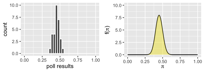
FIGURE 3.1: The results of 30 previous polls of Minnesotans’ support of Michelle for president (left) and a corresponding continuous prior model for \(\pi\), her current election support (right).

Elections are dynamic, thus Michelle’s support is always in flux. Yet these past polls provide prior information about \(\pi\), the proportion of Minnesotans that currently support Michelle. In fact, we can reorganize this information into a formal prior probability model of \(\pi\). We worked a similar example in Section 2.3, in which context \(\pi\) was Kasparov’s probability of beating Deep Blue at chess. In that case, we greatly over-simplified reality to fit within the framework of introductory Bayesian models. Mainly, we assumed that \(\pi\) could only be 0.2, 0.5, or 0.8, the corresponding chances of which were defined by a discrete probability model. However, in the reality of Michelle’s election support and Kasparov’s chess skill, \(\pi\) can be any value between 0 and 1. We can reflect this reality and conduct a more nuanced Bayesian analysis by constructing a continuous prior probability model of \(\pi\). A reasonable prior is represented by the curve in Figure 3.1 (right). We’ll examine continuous models in detail in Section 3.1. For now, simply notice that this curve preserves the overall information and variability in the past polls – Michelle’s support \(\pi\) can be anywhere between 0 and 1, but is most likely around 0.45.

Incorporating this more nuanced, continuous view of Michelle’s support \(\pi\) will require some new tools. BUT the spirit of the Bayesian analysis will remain the same. No matter if our parameter \(\pi\) is continuous or discrete, the posterior model of \(\pi\) will combine insights from the prior and data. Directly ahead, you will dig into the details and build Michelle’s election model. You’ll then generalize this work to the fundamental Beta-Binomial Bayesian model. The power of the Beta-Binomial lies in its broad applications. Michelle’s election support \(\pi\) isn’t the only variable of interest that lives on [0,1]. You might also imagine Bayesian analyses in which we’re interested in modeling the proportion of people that use public transit, the proportion of trains that are delayed, the proportion of people that prefer cats to dogs, and so on. The Beta-Binomial model provides the tools we need to study the proportion of interest, \(\pi\), in each of these settings.

• Utilize and tune continuous priors. You will learn how to interpret and tune a continuous Beta prior model to reflect your prior information about \(\pi\).
• Interpret and communicate features of prior and posterior models using properties such as mean, mode, and variance.
• Construct the fundamental Beta-Binomial model for proportion \(\pi\).

Getting started

To prepare for this chapter, note that we’ll be using three Greek letters throughout our analysis: \(\pi\) = pi, \(\alpha\) = alpha, and \(\beta\) = beta. Further, load the packages below:

library(bayesrules)
library(tidyverse)

3.1 The Beta prior model

In building the Bayesian election model of Michelle’s election support among Minnesotans, \(\pi\), we begin as usual: with the prior. Our continuous prior probability model of \(\pi\) is specified by the probability density function (pdf) in Figure 3.1. Though it looks quite different, the role of this continuous pdf is the same as for the discrete probability mass function (pmf) \(f(\pi)\) in Table 2.7: to specify all possible values of \(\pi\) and the relative plausibility of each. That is, \(f(\pi)\) answers: What values can \(\pi\) take and which are more plausible than others? Further, in accounting for all possible outcomes of \(\pi\), the pdf integrates to or has an area of 1, much like a discrete pmf sums to 1.

Continuous probability models

Let \(\pi\) be a continuous random variable with probability density function \(f(\pi)\). Then \(f(\pi)\) has the following properties:

• \(f(\pi) \ge 0\);
• \(\int_\pi f(\pi)d\pi = 1\), i.e., the area under \(f(\pi)\) is 1; and
• \(P(a < \pi < b) = \int_a^b f(\pi) d\pi\) when \(a \le b\), i.e., the area between any two possible values \(a\) and \(b\) corresponds to the probability of \(\pi\) being in this range.

Interpreting \(f(\pi)\)

It’s possible that \(f(\pi) > 1\), thus a continuous pdf cannot be interpreted as a probability. Rather, \(f(\pi)\) can be used to compare the plausibility of two different values of \(\pi\): the greater \(f(\pi)\), the more plausible the corresponding value of \(\pi\).

NOTE: Don’t fret if integrals are new to you. You will not need to perform any integration to proceed with this book.

3.1.1 Beta foundations

The next step is to translate the picture of our prior in Figure 3.1 (right) into a formal probability model of \(\pi\). That is, we must specify a formula for the pdf \(f(\pi)\). In the world of probability, there are a variety of common “named” models, the pdfs and properties of which are well studied. Among these, it’s natural to focus on the Beta probability model here. Like Michelle’s support \(\pi\), a Beta random variable is continuous and restricted to live on [0,1]. In this section, you’ll explore the properties of the Beta model and how to tune the Beta to reflect our prior understanding of Michelle’s support \(\pi\). Let’s begin with a general definition of the Beta probability model.

The Beta model

Let \(\pi\) be a random variable which can take any value between 0 and 1, i.e., \(\pi \in [0,1]\). Then the variability in \(\pi\) might be well modeled by a Beta model with shape hyperparameters \(\alpha > 0\) and \(\beta > 0\):

\[\pi \sim \text{Beta}(\alpha, \beta).\]

The Beta model is specified by continuous pdf

\[\begin{equation} f(\pi) = \frac{\Gamma(\alpha + \beta)}{\Gamma(\alpha)\Gamma(\beta)} \pi^{\alpha-1} (1-\pi)^{\beta-1} \;\; \text{ for } \pi \in [0,1] \tag{3.1} \end{equation}\] where \(\Gamma(z) = \int_0^\infty x^{z-1}e^{-y}dx\) and \(\Gamma(z + 1) = z \Gamma(z)\). Fun fact: when \(z\) is a positive integer, then \(\Gamma(z)\) simplifies to \(\Gamma(z) = (z-1)!\).

Hyperparameter

A hyperparameter is a parameter used in a prior model.

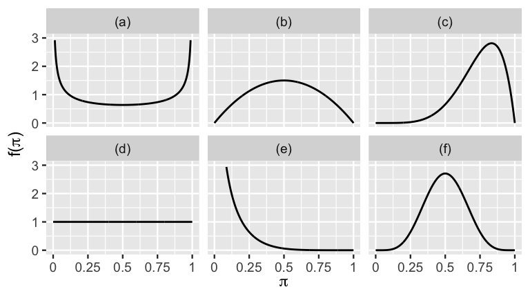
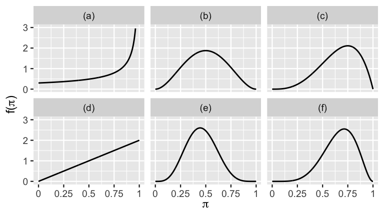
This model is best understood by playing around. Figure 3.2 plots the Beta pdf \(f(\pi)\) under a variety of shape hyperparameters, \(\alpha\) and \(\beta\). Check out the various shapes the Beta pdf can take. This flexibility means that we can tune the Beta to reflect our prior understanding of \(\pi\) by tweaking \(\alpha\) and \(\beta\). For example, notice that when we set \(\alpha = \beta = 1\) (middle left plot), the Beta model is flat from 0 to 1. In this setting, the Beta model is equivalent to perhaps a more familiar model, the standard Uniform.

The standard Uniform model

When it’s equally plausible for \(\pi\) to take on any value between 0 and 1, we can model \(\pi\) by the standard Uniform model

\[\pi \sim \text{Unif}(0,1)\]

with pdf \(f(\pi) = 1\) for \(\pi \in [0,1]\). The Unif(0,1) model is a special case of Beta(\(\alpha,\beta\)) when \(\alpha = \beta = 1\).

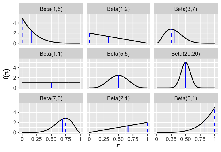
FIGURE 3.2: Beta(\(\alpha,\beta\)) pdfs \(f(\pi)\) under a variety of shape hyperparameters \(\alpha\) and \(\beta\) (black curve). The mean and mode are represented by a blue solid line and dashed line, respectively.

Take a minute to see if you can identify some other patterns in how shape hyperparameters \(\alpha\) and \(\beta\) reflect the typical values of \(\pi\) as well as the variability in \(\pi\).²⁴

1. How would you describe the typical behavior of a Beta(\(\alpha,\beta\)) variable \(\pi\) when \(\alpha = \beta\)?
   a) Right-skewed with \(\pi\) tending to be less than 0.5.
   b) Symmetric with \(\pi\) tending to be around 0.5.
   c) Left-skewed with \(\pi\) tending to be greater than 0.5.

2. Using the same options as above, how would you describe the typical behavior of a Beta(\(\alpha,\beta\)) variable \(\pi\) when \(\alpha > \beta\)?

3. For which model is there greater variability in the plausible values of \(\pi\), Beta(20,20) or Beta(5,5)?

We can support our observations of the behavior in \(\pi\) with numerical measurements. The mean (or “expected value”) and mode of \(\pi\) provide measures of central tendency, or what’s typical. Conceptually speaking, the mean captures the average value of \(\pi\), whereas the mode captures the most plausible value of \(\pi\), i.e., the value of \(\pi\) at which pdf \(f(\pi)\) is maximized. These measures are represented by the solid and dashed vertical lines, respectively, in Figure 3.2. Notice that when \(\alpha\) is less than \(\beta\) (top row), the Beta pdf is right skewed, thus the mean exceeds the mode of \(\pi\) and both are below 0.5. The opposite is true when \(\alpha\) is greater than \(\beta\) (bottom row). When \(\alpha\) and \(\beta\) are equal (center row), the Beta pdf is symmetric around a common mean and mode of 0.5. These trends reflect the formulas for the mean, denoted \(E(\pi)\), and mode for a Beta(\(\alpha, \beta\)) variable \(\pi\):²⁵

\[\begin{equation} \begin{split} E(\pi) & = \frac{\alpha}{\alpha + \beta} \\ \text{Mode}(\pi) & = \frac{\alpha - 1}{\alpha + \beta - 2} \;\;\; \text{ when } \; \alpha, \beta > 1. \\ \end{split} \tag{3.2} \end{equation}\]

For example, the central tendency of a \(\text{Beta}(5,5)\) variable \(\pi\) can be described by

\[E(\pi) = \frac{5}{5 + 5} = 0.5 \;\; \text{ and } \;\; \text{Mode}(\pi) = \frac{5 - 1}{5 + 5 - 2} = 0.5 .\]

Figure 3.2 also reveals patterns in the variability of \(\pi\). For example, with values that tend to be closer to the mean of 0.5, the variability in \(\pi\) is smaller for the Beta(20,20) model than for the Beta(5,5) model. We can measure the variability of a Beta(\(\alpha,\beta\)) random variable \(\pi\) by variance

\[\begin{equation} \text{Var}(\pi) = \frac{\alpha \beta}{(\alpha + \beta)^2(\alpha + \beta + 1)} . \tag{3.3} \end{equation}\]

Roughly speaking, variance measures the typical squared distance of \(\pi\) values from the mean, \(E(\pi)\). Since the variance thus has squared units, it’s typically easier to work with the standard deviation which measures the typical unsquared distance of \(\pi\) values from \(E(\pi)\):

\[\text{SD}(\pi) := \sqrt{\text{Var}(\pi)} .\]

For example, the values of a \(\text{Beta}(5,5)\) variable \(\pi\) tend to deviate from their mean of 0.5 by 0.151, whereas the values of a \(\text{Beta}(20,20)\) variable tend to deviate from 0.5 by only 0.078:

\[\sqrt{\frac{5 \cdot 5}{(5 + 5)^2(5 + 5 + 1)}} = 0.151 \;\;\; \text{ and } \;\;\; \sqrt{\frac{20 \cdot 20}{(20 + 20)^2(20 + 20 + 1)}} = 0.078 .\]

The formulas above don’t magically pop out of nowhere. They are obtained by applying general definitions of mean, mode, and variance to the Beta pdf (3.1). We provide these definitions below, but you can skip them without consequence.

The theory behind measuring central tendency and variability

Let \(\pi\) be a continuous random variable with pdf \(f(\pi)\). Consider two common measures of the central tendency in \(\pi\). The mean or expected value of \(\pi\) captures the weighted average of \(\pi\), where each possible \(\pi\) value is weighted by its corresponding pdf value:
\[E(\pi) = \int \pi \cdot f(\pi)d\pi.\] The mode of \(\pi\) captures the most plausible value of \(\pi\), i.e., the value of \(\pi\) for which the pdf is maximized:

\[\text{Mode}(\pi) = \text{argmax}_\pi f(\pi).\]

Next, consider two common measures of the variability in \(\pi\). The variance in \(\pi\) roughly measures the typical or expected squared distance of possible \(\pi\) values from their mean:

\[\text{Var}(\pi) = E((\pi - E(\pi))^2) = \int (\pi - E(\pi))^2 \cdot f(\pi) d\pi.\]

The standard deviation in \(\pi\) roughly measures the typical or expected distance of possible \(\pi\) values from their mean:

\[\text{SD}(\pi) := \sqrt{\text{Var}(\pi)} .\]

NOTE: If \(\pi\) were discrete with pmf \(f(\pi)\), we’d replace \(\int\) with \(\sum\).

3.1.2 Tuning the Beta prior

With a sense for how the Beta(\(\alpha,\beta\)) model works, let’s tune the shape hyperparameters \(\alpha\) and \(\beta\) to reflect our prior information about Michelle’s election support \(\pi\). We saw in Figure 3.1 (left) that across 30 previous polls, Michelle’s average support was around 45 percentage points, though she roughly polled as low as 25 and as high as 65 percentage points. Our Beta(\(\alpha,\beta\)) prior should have similar patterns. For example, we want to pick \(\alpha\) and \(\beta\) for which \(\pi\) tends to be around 0.45, \(E(\pi) = \alpha/(\alpha + \beta) \approx 0.45\). Or, after some rearranging,

\[\alpha \approx \frac{9}{11} \beta .\]

In a trial and error process, we use plot_beta() in the bayesrules package to plot Beta models with \(\alpha\) and \(\beta\) pairs that meet this constraint (e.g., Beta(9,11), Beta(27,33), Beta(45,55)). Among these, we find that the Beta(45,55) closely captures the typical outcomes and variability in the old polls:

# Plot the Beta(45, 55) prior
plot_beta(45, 55)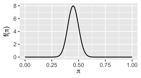

FIGURE 3.3: The Beta(45,55) probability density function.

Thus, a reasonable prior model for Michelle’s election support is

\[\pi \sim \text{Beta}(45,55)\]

with prior pdf \(f(\pi)\) following from plugging 45 and 55 into (3.1),

\[\begin{equation} f(\pi) = \frac{\Gamma(100)}{\Gamma(45)\Gamma(55)}\pi^{44}(1-\pi)^{54} \;\; \text{ for } \pi \in [0,1] . \tag{3.4} \end{equation}\]

By (3.2), this model specifies that Michelle’s election support is most likely around 45 percentage points, with prior mean and prior mode

\[\begin{equation} E(\pi) = \frac{45}{45 + 55} = 0.4500 \;\; \text{ and } \;\; \text{Mode}(\pi) = \frac{45 - 1}{45 + 55 - 2} = 0.4490 . \tag{3.5} \end{equation}\]

Further, by (3.3), the potential variability in \(\pi\) is described by a prior standard deviation of 0.05. That is, our other prior assumptions about Michelle’s possible election support tend to deviate by 5 percentage points from the prior mean of 45%:

\[\begin{equation} \begin{split} \text{Var}(\pi) & = \frac{45 \cdot 55}{(45 + 55)^2(45 + 55 + 1)} = 0.0025 \\ \text{SD}(\pi) & = \sqrt{0.0025} = 0.05.\\ \end{split} \tag{3.6} \end{equation}\]

3.2 The Binomial data model & likelihood function

In the second step of our Bayesian analysis of Michelle’s election support \(\pi\), you’re ready to collect some data. You plan to conduct a new poll of \(n = 50\) Minnesotans and record \(Y\), the number that support Michelle. The results depend upon, and thus will provide insight into, \(\pi\) – the greater Michelle’s actual support, the greater \(Y\) will tend to be. To model the dependence of \(Y\) on \(\pi\), we can make the following assumptions about the poll: 1) voters answer the poll independently of one another; and 2) the probability that any polled voter supports your candidate Michelle is \(\pi\). It follows from our work in Section 2.3.2 that, conditional on \(\pi\), \(Y\) is Binomial. Specifically,

\[Y | \pi \sim \text{Bin}(50, \pi)\]

with conditional pmf \(f(y|\pi)\) defined for \(y \in \{0,1,2,...,50\}\),

\[\begin{equation} f(y|\pi) = P(Y=y | \pi) = \left(\!\!\begin{array}{c} 50 \\ y \end{array}\!\!\right) \pi^y (1-\pi)^{50-y} . \tag{3.7} \end{equation}\]

Given its importance in our Bayesian analysis, it’s worth re-emphasizing the details of the Binomial model. To begin, the conditional pmf \(f(y|\pi)\) provides answers to a hypothetical question: if Michelle’s support were some given value of \(\pi\), then how many of the 50 polled voters \(Y = y\) might we expect to support her? Figure 3.4 plots this pmf under a range of possible \(\pi\). These plots formalize our understanding that if Michelle’s support \(\pi\) were low (top row), the polling result \(Y\) is also likely to be low. If her support were high (bottom row), \(Y\) is also likely to be high.

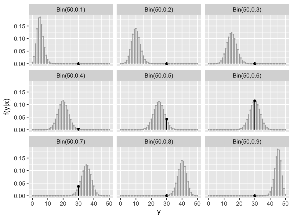
FIGURE 3.4: The Bin(50, \(\pi\)) pmf \(f(y|\pi)\) is plotted for values of \(\pi \in \{0.1, 0.2, \ldots, 0.9\}\). The pmfs at the observed value of polling data \(Y = 30\) are highlighted in black.

In reality, we ultimately observe that the poll was a huge success: \(Y = 30\) of \(n = 50\) (60%) polled voters support Michelle! This result is highlighted by the black lines among the pmfs in Figure 3.4. To focus on just these results that match the observed polling data, we extract and compare these black lines in a single plot (Figure 3.5). These represent the likelihoods of the observed polling data, \(Y = 30\), at each potential level of Michelle’s support \(\pi\) in \(\{0.1,0.2,\ldots,0.9\}\). In fact, this discrete set of scenarios represents a small handful of points along the complete continuous likelihood function \(L(\pi | y=30)\) defined for any \(\pi\) between 0 and 1 (black curve).

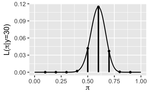
FIGURE 3.5: The likelihood function, \(L(\pi | y = 30)\), of Michelle’s election support \(\pi\) given the observed poll in which \(Y = 30\) of \(n = 50\) polled Minnesotans supported her. The vertical lines represent the likelihood evaluated at \(\pi\) in \(\{0.1,0.2,\ldots,0.9\}\).

Recall that the likelihood function is defined by turning the Binomial pmf on its head. Treating \(Y = 30\) as observed data and \(\pi\) as unknown, matching the reality of our situation, the Binomial likelihood function of \(\pi\) follows from plugging \(y = 30\) into the Binomial pmf (3.7):

\[\begin{equation} L(\pi | y=30) = \left(\!\!\begin{array}{c} 50 \\ 30 \end{array}\!\!\right) \pi^{30} (1-\pi)^{20} \; \; \text{ for } \pi \in [0,1] . \tag{3.8} \end{equation}\]

For example, matching what we see in Figure 3.5, the chance that \(Y = 30\) of 50 polled voters would support Michelle is 0.115 if her underlying support were \(\pi = 0.6\):

\[L(\pi = 0.6 | y = 30) = \left(\!\!\begin{array}{c} 50 \\ 30 \end{array}\!\!\right) 0.6^{30} 0.4^{20} \approx 0.115\]

but only 0.042 if her underlying support were \(\pi = 0.5\):

\[L(\pi = 0.5 | y = 30) = \left(\!\!\begin{array}{c} 50 \\ 30 \end{array}\!\!\right) 0.5^{30} 0.5^{20} \approx 0.042 .\]

It’s also important to remember here that \(L(\pi|y = 30)\) is a function of \(\pi\) that provides insight into the relative compatibility of the observed polling data \(Y = 30\) with different \(\pi \in [0,1]\). The fact that \(L(\pi|y=30)\) is maximized when \(\pi = 0.6\) suggests that the 60% support for Michelle among polled voters is most likely when her underlying support is also at 60%. This makes sense! The further that a hypothetical \(\pi\) value is from 0.6, the less likely we would be to observe our poll result – \(L(\pi | y = 30)\) effectively drops to 0 for \(\pi\) values under 0.3 and above 0.9. Thus, it’s extremely unlikely that we would’ve observed a 60% support rate in the new poll if, in fact, Michelle’s underlying support were as low as 30% or as high as 90%.

3.3 The Beta posterior model

We now have two pieces of our Bayesian model in place – the Beta prior model for Michelle’s support \(\pi\) and the Binomial model for the dependence of polling data \(Y\) on \(\pi\):

\[\begin{split} Y | \pi & \sim \text{Bin}(50, \pi) \\ \pi & \sim \text{Beta}(45, 55). \\ \end{split}\]

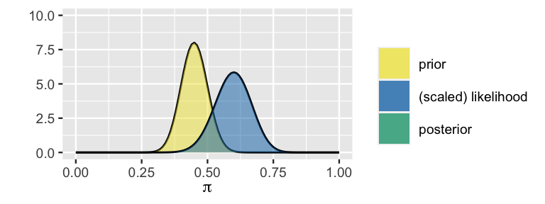
FIGURE 3.6: The prior model of \(\pi\) along with the (scaled) likelihood function of \(\pi\) given the new poll results in which \(Y = 30\) of \(n = 50\) polled Minnesotans support Michelle.

These pieces of the puzzle are shown together in Figure 3.6 where, only for the purposes of visual comparison to the prior, the likelihood function is scaled to integrate to 1.²⁶ The prior and data, as captured by the likelihood, don’t completely agree. Constructed from old polls, the prior is a bit more pessimistic about Michelle’s election support than the data obtained from the latest poll. Yet both insights are valuable to our analysis. Just as much as we shouldn’t ignore the new poll in favor of the old, we also shouldn’t throw out our bank of prior information in favor of the newest thing (also great life advice). Thinking like Bayesians, we can construct a posterior model of \(\pi\) which combines the information from the prior with that from the data.

Which plot reflects the correct posterior model of Michelle’s election support \(\pi\)?

Plot (b) is the only plot in which the posterior model of \(\pi\) strikes a balance between the relative pessimism of the prior and optimism of the data. You can reproduce this correct posterior using the plot_beta_binomial() function in the bayesrules package, plugging in the prior hyperparameters \((\alpha = 45, \beta = 55\)) and data (\(y = 30\) of \(n = 50\) polled voters support Michelle):

plot_beta_binomial(alpha = 45, beta = 55, y = 30, n = 50)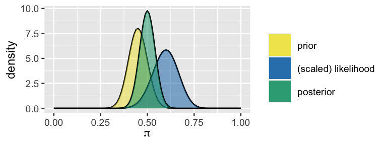

FIGURE 3.7: The prior pdf, scaled likelihood function, and posterior pdf of Michelle’s election support \(\pi\).

In its balancing act, the posterior here is slightly “closer” to the prior than to the likelihood. (We’ll gain intuition for why this is the case in Chapter 4.) The posterior being centered at \(\pi = 0.5\) suggests that Michelle’s support is equally likely to be above or below the 50% threshold required to win Minnesota. Further, combining information from the prior and data, the range of posterior plausible values has narrowed: we can be fairly certain that Michelle’s support is somewhere between 35% and 65%.

You might also recognize something new: like the prior, the posterior model of \(\pi\) is continuous and lives on [0,1]. That is, like the prior, the posterior appears to be a Beta(\(\alpha,\beta\)) model where the shape parameters have been updated to combine information from the prior and data. This is indeed the case. Conditioned on the observed poll results (\(Y = 30\)), the posterior model of Michelle’s election support is Beta(75, 75):

\[\pi | (Y = 30) \sim \text{Beta}(75,75)\]

with a corresponding pdf which follows from (3.1):

\[\begin{equation} f(\pi | y = 30) = \frac{\Gamma(150)}{\Gamma(75)\Gamma(75)}\pi^{74} (1-\pi)^{74} \;\; \text{ for } \pi \in [0,1] . \tag{3.9} \end{equation}\]

Before backing up this claim with some math, let’s examine the evolution in your understanding of Michelle’s election support \(\pi\). The summarize_beta_binomial() function in the bayesrules package summarizes the typical values and variability in the prior and posterior models of \(\pi\). These calculations follow directly from applying the prior and posterior Beta parameters into (3.2) and (3.3):

summarize_beta_binomial(alpha = 45, beta = 55, y = 30, n = 50)
      model alpha beta mean  mode      var      sd
1     prior    45   55 0.45 0.449 0.002450 0.04950
2 posterior    75   75 0.50 0.500 0.001656 0.04069

A comparison illuminates the polling data’s influence on the posterior model. Mainly, after observing the poll in which 30 of 50 people supported Michelle, the expected value of her underlying support \(\pi\) nudged up from approximately 45% to 50%:

\[E(\pi) = 0.45 \;\; \text{ vs } \;\; E(\pi | Y = 30) = 0.50 .\]

Further, the variability within the model decreased, indicating a narrower range of posterior plausible \(\pi\) values in light of the polling data:

\[\text{SD}(\pi) \approx 0.0495 \;\; \text{ vs } \;\; \text{SD}(\pi | Y = 30) \approx 0.0407 .\]

If you’re happy taking our word that the posterior model of \(\pi\) is Beta(75,75), you can skip to Section 3.4 and still be prepared for the next material in the book. However, we strongly recommend that you consider the magic from which the posterior is built. Going through the process can help you further develop intuition for Bayesian modeling. As with our previous Bayesian models, the posterior conditional pdf of \(\pi\) strikes a balance between the prior pdf \(f(\pi)\) and the likelihood function \(L(\pi|y = 30)\) via Bayes’ Rule (2.12):

\[f(\pi | y = 30) = \frac{f(\pi)L(\pi|y = 30)}{f(y = 30)}.\]

Recall from Section 2.3.6 that \(f(y = 30)\) is a normalizing constant, i.e., a constant across \(\pi\) which scales the posterior pdf \(f(\pi | y = 30)\) to integrate to 1. We don’t need to calculate the normalizing constant in order to construct the posterior model. Rather, we can simplify the posterior construction by utilizing the fact that the posterior pdf is proportional to the product of the prior pdf (3.4) and likelihood function (3.8):

\[\begin{split} f(\pi | y = 30) & \propto f(\pi) L(\pi | y=30) \\ & = \frac{\Gamma(100)}{\Gamma(45)\Gamma(55)}\pi^{44}(1-\pi)^{54} \cdot \left(\!\!\begin{array}{c} 50 \\ 30 \end{array}\!\!\right) \pi^{30} (1-\pi)^{20} \\ & = \left[\frac{\Gamma(100)}{\Gamma(45)\Gamma(55)}\left(\!\!\begin{array}{c} 50 \\ 30 \end{array}\!\!\right) \right] \cdot \pi^{74} (1-\pi)^{74} \\ & \propto \pi^{74} (1-\pi)^{74} . \\ \end{split}\]

In the third line of our calculation, we combined the constants and the elements that depend upon \(\pi\) into two different pieces. In the final line, we made a big simplification: we dropped all constants that don’t depend upon \(\pi\). We don’t need these. Rather, it’s the dependence of \(f(\pi | y=30)\) on \(\pi\) that we care about:

\[f(\pi | y=30) = c\pi^{74} (1-\pi)^{74} \propto \pi^{74} (1-\pi)^{74} .\]

We could complete the definition of this posterior pdf by calculating the normalizing constant \(c\) for which the pdf integrates to 1:

\[1 = \int f(\pi | y=30) d\pi = \int c \cdot \pi^{74} (1-\pi)^{74} d\pi \;\; \Rightarrow \; \; c = \frac{1}{\int \pi^{74} (1-\pi)^{74} d\pi}.\] But again, we don’t need to do this calculation. The pdf of \(\pi\) is defined by its structural dependence on \(\pi\), that is, the kernel of the pdf. Notice here that \(f(\pi|y=30)\) has the same kernel as the normalized Beta(75,75) pdf in (3.9):

\[f(\pi | y=30) = \frac{\Gamma(150)}{\Gamma(75)\Gamma(75)} \pi^{74} (1-\pi)^{74} \propto \pi^{74} (1-\pi)^{74} .\]

The fact that the unnormalized posterior pdf \(f(\pi | y=30)\) matches an unnormalized Beta(75,75) pdf verifies our claim that \(\pi | (Y=30) \sim \text{Beta}(75,75)\). Magic. For extra practice in identifying the posterior model of \(\pi\) from an unnormalized posterior pdf or kernel, take the following quiz.²⁷

For each scenario below, identify the correct Beta posterior model of \(\pi \in [0,1]\) from its unnormalized pdf.

1. \(f(\pi|y) \propto \pi^{3 - 1}(1-\pi)^{12 - 1}\)
2. \(f(\pi|y) \propto \pi^{11}(1-\pi)^{2}\)
3. \(f(\pi|y) \propto 1\)

Now, instead of identifying a model from a kernel, practice identifying the kernels of models.²⁸

Identify the kernels of each pdf below.

1. \(f(\pi|y) = ye^{-\pi y}\) for \(\pi > 0\)
   1. \(y\)
   2. \(e^{-\pi}\)
   3. \(ye^{-\pi}\)
   4. \(e^{-\pi y}\)
2. \(f(\pi|y) = \frac{2^y}{(y-1)!} \pi^{y-1}e^{-2\pi}\) for \(\pi > 0\)
   1. \(\pi^{y-1}e^{-2\pi}\)
   2. \(\frac{2^y}{(y-1)!}\)
   3. \(e^{-2\pi}\)
   4. \(\pi^{y-1}\)
3. \(f(\pi) = 3\pi^2\) for \(\pi \in [0,1]\)

3.4 The Beta-Binomial model

In the previous section we developed the fundamental Beta-Binomial model for Michelle’s election support \(\pi\). In doing so, we assumed a specific Beta(45,55) prior and a specific polling result (\(Y=30\) of \(n=50\) polled voters supported your candidate) within a specific context. This was a special case of the more general Beta-Binomial model:

\[\begin{split} Y | \pi & \sim \text{Bin}(n, \pi) \\ \pi & \sim \text{Beta}(\alpha, \beta). \\ \end{split}\]

This general model has vast applications, applying to any setting having a parameter of interest \(\pi\) that lives on [0,1] with any tuning of a Beta prior and any data \(Y\) which is the number of “successes” in \(n\) fixed, independent trials, each having probability of success \(\pi\). For example, \(\pi\) might be a coin’s tendency toward Heads and data \(Y\) records the number of Heads observed in a series of \(n\) coin flips. Or \(\pi\) might be the proportion of adults that use social media and we learn about \(\pi\) by sampling \(n\) adults and recording the number \(Y\) that use social media. No matter the setting, upon observing \(Y = y\) successes in \(n\) trials, the posterior of \(\pi\) can be described by a Beta model which reveals the influence of the prior (through \(\alpha\) and \(\beta\)) and data (through \(y\) and \(n\)):

\[\begin{equation} \pi | (Y = y) \sim \text{Beta}(\alpha + y, \beta + n - y) . \tag{3.10} \end{equation}\]

Measures of posterior central tendency and variability follow from (3.2) and (3.3):

\[\begin{equation} \begin{split} E(\pi | Y=y) & = \frac{\alpha + y}{\alpha + \beta + n} \\ \text{Mode}(\pi | Y=y) & = \frac{\alpha + y - 1}{\alpha + \beta + n - 2} \\ \text{Var}(\pi | Y=y) & = \frac{(\alpha + y)(\beta + n - y)}{(\alpha + \beta + n)^2(\alpha + \beta + n + 1)}.\\ \end{split} \tag{3.11} \end{equation}\]

Importantly, notice that the posterior follows a different parameterization of the same probability model as the prior – both the prior and posterior are Beta models with different tunings. In this case, we say that the Beta(\(\alpha, \beta\)) model is a conjugate prior for the corresponding Bin(\(n,\pi\)) data model. Our work below will highlight that conjugacy simplifies the construction of the posterior, and thus can be a desirable property in Bayesian modeling.

Conjugate prior

We say that \(f(\pi)\) is a conjugate prior for \(L(\pi|y)\) if the posterior, \(f(\pi|y) \propto f(\pi)L(\pi|y)\), is from the same model family as the prior.

The posterior construction for the general Beta-Binomial model is very similar to that of the election-specific model. First, the Beta prior pdf \(f(\pi)\) is defined by (3.1) and the likelihood function \(L(\pi|y)\) by (2.7), the conditional pmf of the Bin(\(n,\pi\)) model upon observing data \(Y = y\). For \(\pi \in [0,1]\),

\[\begin{equation} f(\pi) = \frac{\Gamma(\alpha + \beta)}{\Gamma(\alpha)\Gamma(\beta)}\pi^{\alpha - 1}(1-\pi)^{\beta - 1} \;\; \text{ and } \;\; L(\pi|y) = \left(\!\!\begin{array}{c} n \\ y \end{array}\!\!\right) \pi^{y} (1-\pi)^{n-y} . \tag{3.12} \end{equation}\]

Putting these two pieces together, the posterior pdf follows from Bayes’ Rule:

\[\begin{split} f(\pi | y) & \propto f(\pi)L(\pi|y) \\ & = \frac{\Gamma(\alpha + \beta)}{\Gamma(\alpha)\Gamma(\beta)}\pi^{\alpha - 1}(1-\pi)^{\beta - 1} \cdot \left(\!\begin{array}{c} n \\ y \end{array}\!\right) \pi^{y} (1-\pi)^{n-y} \\ & \propto \pi^{(\alpha + y) - 1} (1-\pi)^{(\beta + n - y) - 1} .\\ \end{split}\]

Again, we’ve dropped normalizing constants which don’t depend upon \(\pi\) and are left with the unnormalized posterior pdf. Note that this shares the same structure as the normalized Beta(\(\alpha + y\), \(\beta + n - y\)) pdf,

\[f(\pi|y) = \frac{\Gamma(\alpha+\beta+n)}{\Gamma(\alpha+y)\Gamma(\beta+n-y)}\pi^{(\alpha + y) - 1} (1-\pi)^{(\beta + n - y) - 1}.\]

Thus, we’ve verified our claim that the posterior model of \(\pi\) given an observed \(Y = y\) successes in \(n\) trials is \(\text{Beta}(\alpha + y, \beta + n - y)\).

3.5 Simulating the Beta-Binomial

Using Section 2.3.7 as a guide, let’s simulate the posterior model of Michelle’s support \(\pi\). We begin by simulating 10,000 values of \(\pi\) from the Beta(45,55) prior using rbeta() and, subsequently, a potential Bin(50,\(\pi\)) poll result \(Y\) from each \(\pi\) using rbinom():

set.seed(84735)
michelle_sim <- data.frame(pi = rbeta(10000, 45, 55)) %>% 
  mutate(y = rbinom(10000, size = 50, prob = pi))

The resulting 10,000 pairs of \(\pi\) and \(y\) values are shown in Figure 3.8. In general, the greater Michelle’s support, the better her poll results tend to be. Further, the highlighted pairs illustrate that the eventual observed poll result, \(Y = 30\) of 50 polled voters supported Michelle, would most likely arise if her underlying support \(\pi\) were somewhere in the range from 0.4 to 0.6.

ggplot(michelle_sim, aes(x = pi, y = y)) + 
  geom_point(aes(color = (y == 30)), size = 0.1)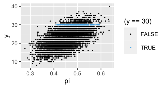

FIGURE 3.8: A scatterplot of 10,000 simulated pairs of Michelle’s support \(\pi\) and polling outcome \(y\).

When we zoom in closer on just those pairs that match our \(Y = 30\) poll results, the behavior across the remaining set of \(\pi\) values well approximates the Beta(75,75) posterior model of \(\pi\):

# Keep only the simulated pairs that match our data
michelle_posterior <- michelle_sim %>% 
  filter(y == 30)

# Plot the remaining pi values
ggplot(michelle_posterior, aes(x = pi)) + 
  geom_density()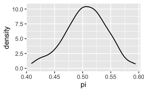

FIGURE 3.9: A density plot of simulated \(\pi\) values that produced polling outcomes in which \(Y = 30\) voters supported Michelle.

As such, we can also use our simulated sample to approximate posterior features, such as the mean and standard deviation in Michelle’s support. The results are quite similar to the theoretical values calculated above, \(E(\pi | Y = 30) = 0.5\) and \(\text{SD}(\pi | Y = 30) = 0.0407\):

michelle_posterior %>% 
  summarize(mean(pi), sd(pi))
  mean(pi)  sd(pi)
1   0.5055 0.03732

In interpreting these simulation results, “approximate” is a key word. Since only 211 of our 10,000 simulations matched our observed \(Y = 30\) data, this approximation might be improved by upping our original simulations from 10,000 to, say, 50,000:

nrow(michelle_posterior)
[1] 211

3.6 Example: Milgram’s behavioral study of obedience

In a 1963 issue of The Journal of Abnormal and Social Psychology, Stanley Milgram described a study in which he investigated the propensity of people to obey orders from authority figures, even when those orders may harm other people (Milgram 1963). In the paper, Milgram describes the study as:

“consist[ing] of ordering a naive subject to administer electric shock to a victim. A simulated shock generator is used, with 30 clearly marked voltage levels that range from IS to 450 volts. The instrument bears verbal designations that range from Slight Shock to Danger: Severe Shock. The responses of the victim, who is a trained confederate of the experimenter, are standardized. The orders to administer shocks are given to the naive subject in the context of a `learning experiment’ ostensibly set up to study the effects of punishment on memory. As the experiment proceeds the naive subject is commanded to administer increasingly more intense shocks to the victim, even to the point of reaching the level marked Danger: Severe Shock.”

In other words, study participants were given the task of testing another participant (who was in truth a trained actor) on their ability to memorize facts. If the actor didn’t remember a fact, the participant was ordered to administer a shock on the actor and to increase the shock level with every subsequent failure. Unbeknownst to the participant, the shocks were fake and the actor was only pretending to register pain from the shock.

3.6.1 A Bayesian analysis

We can translate Milgram’s study into the Beta-Binomial framework. The parameter of interest here is \(\pi\), the chance that a person would obey authority (in this case, administering the most severe shock), even if it meant bringing harm to others. Since Milgram passed away in 1984, we don’t have the opportunity to ask him about his understanding of \(\pi\) prior to conducting the study. Thus, we’ll diverge from the actual study here, and suppose that another psychologist helped carry out this work. Prior to collecting data, they indicated that a Beta(1,10) model accurately reflected their understanding about \(\pi\), developed through previous work. Next, let \(Y\) be the number of the 40 study participants that would inflict the most severe shock. Assuming that each participant behaves independently of the others, we can model the dependence of \(Y\) on \(\pi\) using the Binomial. In summary, we have the following Beta-Binomial Bayesian model:

\[\begin{split} Y | \pi & \sim \text{Bin}(40, \pi) \\ \pi & \sim \text{Beta}(1,10) . \\ \end{split}\]

Before moving ahead with our analysis, let’s examine the psychologist’s prior model.

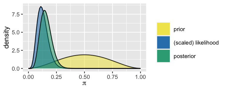
What does the Beta(1,10) prior model in Figure 3.10 reveal about the psychologist’s prior understanding of \(\pi\)?

1. They don’t have an informed opinion.
2. They’re fairly certain that a large proportion of people will do what authority tells them.
3. They’re fairly certain that only a small proportion of people will do what authority tells them.

# Beta(1,10) prior
plot_beta(alpha = 1, beta = 10)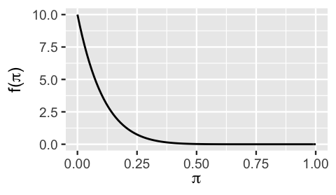

FIGURE 3.10: A Beta(1,10) prior model of \(\pi\).

The correct answer to this quiz is c. The psychologist’s prior is that \(\pi\) typically takes on values near 0 with low variability. Thus, the psychologist is fairly certain that very few people will just do whatever authority tells them. Of course, the psychologist’s understanding will evolve upon seeing the results of Milgram’s study.

In the end, 26 of the 40 study participants inflicted what they understood to be the maximum shock. In light of this data, what’s the psychologist’s posterior model of \(\pi\):

\[\pi | (Y = 26) \sim \text{Beta}(\text{???}, \text{???})\]

Plugging the prior hyperparameters (\(\alpha = 1\), \(\beta = 10\)) and data (\(y = 26\), \(n = 40\)) into (3.10) establishes the psychologist’s posterior model of \(\pi\):

\[\pi | (Y = 26) \sim \text{Beta}(27, 24) .\]

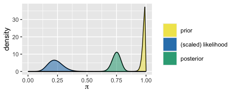
This posterior is summarized and plotted below, contrasted with the prior pdf and scaled likelihood function. Note that the psychologist’s understanding evolved quite a bit from their prior to their posterior. Though they started out with an understanding that fewer than ~25% of people would inflict the most severe shock, given the strong counterevidence in the study data, they now understand this figure to be somewhere between ~30% and ~70%.

summarize_beta_binomial(alpha = 1, beta = 10, y = 26, n = 40)
      model alpha beta    mean   mode      var      sd
1     prior     1   10 0.09091 0.0000 0.006887 0.08299
2 posterior    27   24 0.52941 0.5306 0.004791 0.06922

plot_beta_binomial(alpha = 1, beta = 10, y = 26, n = 40)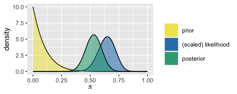

FIGURE 3.11: The Beta prior pdf, scaled Binomial likelihood function, and Beta posterior pdf for \(\pi\), the proportion of subjects that would follow the given instructions.

3.6.2 The role of ethics in statistics and data science

In working through the previous example, we hope you were a bit distracted by your inner voice – this experiment seems ethically dubious. You wouldn’t be alone in this thinking. Stanley Milgram is a controversial historical figure. We chose the above example to not only practice building Beta-Binomial models, but to practice taking a critical eye to our work and the work of others. Every data collection, visualization, analysis, and communication engenders both harms and benefits to individuals and groups, both direct and indirect. As statisticians and data scientists, it is critical to always consider these harms and benefits. We encourage you to ask yourself the following questions each time you work with data:

• What are the study’s potential benefits to society? To participants?
• What are the study’s potential risks to society? To participants?
• What ethical issues might arise when generalizing observations on the study participants to a larger population?
• Who is included and excluded in this study? What are the corresponding risks and benefits? Are individuals in groups that have been historically (and currently) marginalized put at greater risk?
• Were the people who might be affected by your study involved in the study? If not, you may not be qualified to evaluate these questions.
• What’s the personal story or experience of each subject represented by a row of data?

The importance of considering the context and implications for your statistical and data science work cannot be overstated. As statisticians and data scientists, we are responsible for considering these issues so as not to harm individuals and communities of people. Fortunately, there are many resources available to learn more. To name just a few: Race After Technology (Benjamin 2019), Data Feminism (D’Ignazio and Klein 2020), Algorithms of Oppression (Noble 2018), Datasheets for Datasets (Gebru et al. 2018), Model Cards for Model Reporting (Mitchell et al. 2019), Automating Inequality: How High-Tech Tools Profile, Police, and Punish the Poor (Eubanks 2018), Closing the AI Accountability Gap (Raji et al. 2020), and “Integrating Data Science Ethics Into an Undergraduate Major” (Baumer et al. 2020).

3.7 Chapter summary

In Chapter 3, you built the foundational Beta-Binomial model for \(\pi\), an unknown proportion that can take any value between 0 and 1:

\[\begin{split} Y | \pi & \sim \text{Bin}(n, \pi) \\ \pi & \sim \text{Beta}(\alpha, \beta) \\ \end{split} \;\; \Rightarrow \;\; \pi | (Y = y) \sim \text{Beta}(\alpha + y, \beta + n - y) .\]

This model reflects the four pieces common to every Bayesian analysis:

1. Prior model
   The Beta prior model for \(\pi\) can be tuned to reflect the relative prior plausibility of each \(\pi \in [0,1]\).

\[f(\pi) = \frac{\Gamma(\alpha + \beta)}{\Gamma(\alpha)\Gamma(\beta)}\pi^{\alpha - 1}(1-\pi)^{\beta - 1}.\]

2. Data model
   To learn about \(\pi\), we collect data \(Y\), the number of successes in \(n\) independent trials, each having probability of success \(\pi\). The dependence of \(Y\) on \(\pi\) is summarized by the Binomial model \(\text{Bin}(n,\pi)\).

3. Likelihood function
   Upon observing data \(Y = y\) where \(y \in \{0,1,\ldots,n\}\), the likelihood function of \(\pi\), obtained by plugging \(y\) into the Binomial pmf, provides a mechanism by which to compare the compatibility of the data with different \(\pi\):

   \[L(\pi|y) = \left(\!\begin{array}{c} n \\ y \end{array}\!\right) \pi^{y} (1-\pi)^{n-y} \;\; \text{ for } \pi \in [0,1].\]

4. Posterior model
   Via Bayes’ Rule, the conjugate Beta prior combined with the Binomial data model produce a Beta posterior model for \(\pi\). The updated Beta posterior parameters \((\alpha + y, \beta + n - y)\) reflect the influence of the prior (via \(\alpha\) and \(\beta\)) and the observed data (via \(y\) and \(n\)).

\[f(\pi | y) \propto f(\pi)L(\pi|y) \propto \pi^{(\alpha + y) - 1} (1-\pi)^{(\beta + n - y) - 1} .\]

3.8 Exercises

3.8.1 Practice: Beta prior models

Exercise 3.1 (Tune your Beta prior: Take I) In each situation below, tune a Beta(\(\alpha,\beta\)) model that accurately reflects the given prior information. In many cases, there’s no single “right” answer, but rather multiple “reasonable” answers.

1. Your friend applied to a job and tells you: “I think I have a 40% chance of getting the job, but I’m pretty unsure.” When pressed further, they put their chances between 20% and 60%.
2. A scientist has created a new test for a rare disease. They expect that the test is accurate 80% of the time with a variance of 0.05.
3. Your Aunt Jo is a successful mushroom hunter. She boasts: “I expect to find enough mushrooms to feed myself and my co-workers at the auto-repair shop 90% of the time, but if I had to give you a likely range it would be between 85% and 100% of the time.”
4. Sal (who is a touch hyperbolic) just interviewed for a job, and doesn’t know how to describe their chances of getting an offer. They say, “I couldn’t read my interviewer’s expression! I either really impressed them and they are absolutely going to hire me, or I made a terrible impression and they are burning my resumé as we speak.”

Exercise 3.2 (Tune your Beta prior: Take II) As in Exercise 3.1, tune an appropriate Beta(\(\alpha,\beta\)) prior model for each situation below.

1. Your friend tells you “I think that I have a 80% chance of getting a full night of sleep tonight, and I am pretty certain.” When pressed further, they put their chances between 70% and 90%.
2. A scientist has created a new test for a rare disease. They expect that it’s accurate 90% of the time with a variance of 0.08.
3. Max loves to play the video game Animal Crossing. They tell you: “The probability that I play Animal Crossing in the morning is somewhere between 75% and 95%, but most likely around 85%.”
4. The bakery in Easthampton, Massachusetts often runs out of croissants on Sundays. Ben guesses that by 10 a.m., there is a 30% chance they have run out, but is pretty unsure about that guess.

Exercise 3.3 (It’s OK to admit you don’t know) You want to specify a Beta prior for a situation in which you have no idea about some parameter \(\pi\). You think \(\pi\) is equally likely to be anywhere between 0 and 1.

1. Specify and plot the appropriate Beta prior model.
2. What is the mean of the Beta prior that you specified? Explain why that does or does not align with having no clue.
3. What is the standard deviation of the Beta prior that you specified?
4. Specify and plot an example of a Beta prior that has a smaller standard deviation than the one you specified.
5. Specify and plot an example of a Beta prior that has a larger standard deviation than the one you specified.

Exercise 3.4 (Which Beta? Take I) Six Beta pdfs are plotted below. Match each to one of the following models: Beta(0.5,0.5), Beta(1,1), Beta(2,2), Beta(6,6), Beta(6,2), Beta(0.5,6).

Exercise 3.5 (Which Beta? Take II) Six Beta pdfs are plotted below. Match each to one of the following models: Beta(1,0.3), Beta(2,1), Beta(3,3), Beta(6,3), Beta(4,2), Beta(5,6).

Exercise 3.6 (Beta properties) Examine the properties of the Beta models in Exercise 3.4.

1. Which Beta model has the smallest mean? The biggest? Provide visual evidence and calculate the corresponding means.
2. Which Beta model has the smallest mode? The biggest? Provide visual evidence and calculate the corresponding modes.
3. Which Beta model has the smallest standard deviation? The biggest? Provide visual evidence and calculate the corresponding standard deviations.

Exercise 3.7 (Using R for Beta)

1. Use plot_beta() to plot the six Beta models in Exercise 3.4.
2. Use summarize_beta() to confirm your answers to Exercise 3.6.

Exercise 3.8 (Calculus challenge: establishing Beta features) Let \(\pi\) follow a Beta(\(\alpha, \beta\)) model. Formulas for the mean, mode, and variance of \(\pi\) are given by (3.2) and (3.3). Confirm these properties by applying the following definitions of mean, mode, and variance directly to the Beta pdf \(f(\pi)\), (3.1):

\[\begin{split} E(\pi) & = \int \pi f(\pi) d\pi \\ \text{Mode}(\pi) & = \text{argmax}_\pi f(\pi) \\ \text{Var}(\pi) & = E\left[(\pi - E(\pi))^2\right] = E(\pi^2) - \left[E(\pi)\right]^2. \\ \end{split}\]

Exercise 3.9 (Interpreting priors) What do you call a sweet carbonated drink: pop, soda, coke, or something else? Let \(\pi\) be the proportion of U.S. residents that prefer the term “pop.” Two different beverage salespeople from different regions of the country have different priors for \(\pi\). The first salesperson works in North Dakota and specifies a Beta(8,2) prior. The second works in Louisiana and specifies a Beta(1,20) prior.

1. Calculate the prior mean, mode, standard deviation of \(\pi\) for both salespeople.
2. Plot the prior pdfs for both salespeople.
3. Compare, in words, the salespeople’s prior understandings about the proportion of U.S. residents that say “pop.”

3.8.2 Practice: Beta-Binomial models

Exercise 3.10 (Different priors, different posteriors) Continuing Exercise 3.9, we poll 50 U.S. residents and 12 (24%) prefer the term “pop.”

1. Specify the unique posterior model of \(\pi\) for both salespeople. We encourage you to construct these posteriors from scratch.
2. Plot the prior pdf, likelihood function, and posterior pdf for both salespeople.
3. Compare the salespeople’s posterior understanding of \(\pi\).

Exercise 3.11 (Regular bike ridership) A university wants to know what proportion of students are regular bike riders, \(\pi\), so that they can install an appropriate number of bike racks. Since the university is in sunny Southern California, staff think that \(\pi\) has a mean of 1 in 4 students, and a mode of 5/22.

1. Specify and plot a Beta model that reflects the staff’s prior ideas about \(\pi\).
2. Among 50 surveyed students, 15 are regular bike riders. What is the posterior model for \(\pi\)?
3. What is the mean, mode, and standard deviation of the posterior model?
4. Does the posterior model more closely reflect the prior information or the data? Explain your reasoning.

Exercise 3.12 (Same-sex marriage) A 2017 Pew Research survey found that 10.2% of LGBT adults in the U.S. were married to a same-sex spouse.²⁹ Now it’s the 2020s, and Bayard guesses that \(\pi\), the percent of LGBT adults in the U.S. who are married to a same-sex spouse, has most likely increased to about 15% but could reasonably range from 10% to 25%.

1. Identify and plot a Beta model that reflects Bayard’s prior ideas about \(\pi\).
2. Bayard wants to update his prior, so he randomly selects 90 US LGBT adults and 30 of them are married to a same-sex partner. What is the posterior model for \(\pi\)?
3. Calculate the posterior mean, mode, and standard deviation of \(\pi\).
4. Does the posterior model more closely reflect the prior information or the data? Explain your reasoning.

Exercise 3.13 (Knowing someone who is transgender) A September 2016 Pew Research survey found that 30% of U.S. adults are aware that they know someone who is transgender.³⁰ It is now the 2020s, and Sylvia believes that the current percent of people who know someone who is transgender, \(\pi\), has increased to somewhere between 35% and 60%.

1. Identify and plot a Beta model that reflects Sylvia’s prior ideas about \(\pi\).
2. Sylvia wants to update her prior, so she randomly selects 200 US adults and 80 of them are aware that they know someone who is transgender. Specify and plot the posterior model for \(\pi\).
3. What is the mean, mode, and standard deviation of the posterior model?
4. Describe how the prior and posterior Beta models compare.

Exercise 3.14 (Summarizing the Beta-Binomial: Take I) Write the corresponding input code for the summarize_beta_binomial() output below.

      model alpha beta   mean   mode      var      sd
1     prior     2    3 0.4000 0.3333 0.040000 0.20000
2 posterior    11   24 0.3143 0.3030 0.005986 0.07737

Exercise 3.15 (Summarizing the Beta-Binomial: Take II) Write the corresponding input code for the summarize_beta_binomial() output below.

      model alpha beta   mean   mode       var      sd
1     prior     1    2 0.3333 0.0000 0.0555556 0.23570
2 posterior   100    3 0.9709 0.9802 0.0002719 0.01649

Exercise 3.16 (Plotting the Beta-Binomial: Take I) Below is output from plot_beta_binomial() function.

1. Describe and compare both the prior model and likelihood function in words.
2. Describe the posterior model in words. Does it more closely agree with the data (as reflected by the likelihood function) or the prior?
3. Provide the specific plot_beta_binomial() code you would use to produce a similar plot.

Exercise 3.17 (Plotting the Beta-Binomial: Take II) Repeat Exercise 3.16 for the plot_beta_binomial() output below.

Exercise 3.18 (More Beta-Binomial)

1. Patrick has a Beta(3,3) prior for \(\pi\), the probability that someone in their town attended a protest in June 2020. In their survey of 40 residents, 30 attended a protest. Summarize Patrick’s analysis using summarize_beta_binomial() and plot_beta_binomial().
2. Harold has the same prior as Patrick, but lives in a different town. In their survey, 15 out of 20 people attended a protest. Summarize Harold’s analysis using summarize_beta_binomial() and plot_beta_binomial().
3. How do Patrick and Harold’s posterior models compare? Briefly explain what causes these similarities and differences.

References

Baumer, Benjamin S., Randi L. Garcia, Albert Y. Kim, Katherine M. Kinnaird, and Miles Q. Ott. 2020. “Integrating Data Science Ethics into an Undergraduate Major.” arXiv Preprint arXiv:2001.07649.

Benjamin, Ruha. 2019. Race After Technology: Abolitionist Tools for the New Jim Code. John Wiley & Sons.

D’Ignazio, Catherine, and Lauren F Klein. 2020. Data Feminism. MIT Press.

Eubanks, Virginia. 2018. Automating Inequality: How High-Tech Tools Profile, Police, and Punish the Poor. St. Martin’s Press.

Gebru, Timnit, Jamie Morgenstern, Briana Vecchione, Jennifer Wortman Vaughan, Hanna Wallach, Hal Daumé III, and Kate Crawford. 2018. “Datasheets for Datasets.” arXiv Preprint arXiv:1803.09010.

Milgram, Stanley. 1963. “Behavioral Study of Obedience.” Journal of Abnormal and Social Psychology 67: 371–78.

Mitchell, Margaret, Simone Wu, Andrew Zaldivar, P. Barnes, Lucy Vasserman, B. Hutchinson, Elena Spitzer, Inioluwa Deborah Raji, and Timnit Gebru. 2019. “Model Cards for Model Reporting.” Proceedings of the Conference on Fairness, Accountability, and Transparency.

Noble, Safiya Umoja. 2018. Algorithms of Oppression: How Search Engines Reinforce Racism. NYU Press.

Raji, Inioluwa Deborah, Andrew Smart, Rebecca N White, Margaret Mitchell, Timnit Gebru, Ben Hutchinson, Jamila Smith-Loud, Daniel Theron, and Parker Barnes. 2020. “Closing the AI Accountability Gap: Defining an End-to-End Framework for Internal Algorithmic Auditing.” In Proceedings of the 2020 Conference on Fairness, Accountability, and Transparency, 33–44.

---

24. Answers: 1. b; 2. c; 3. Beta(5,5)↩︎

25. The mode when either \(\alpha \le 1\) or \(\beta \le 1\) is evident from a plot of the pdf.↩︎

26. The scaled likelihood function is calculated by \(L(\pi|y) / \int_0^1 L(\pi|y)d\pi\).↩︎

27. Answer: a. Beta(3,12); b. Beta(12,3); c. Beta(1,1) or, equivalently, Unif(0,1)↩︎

28. Answers: 1. d; 2. a; 3. \(\pi^2\)↩︎

29. https://news.gallup.com/poll/212702/lgbt-adults-married-sex-spouse.aspx?utm_source=alert&utm_medium=email&utm_content=morelink&utm_campaign=syndication↩︎

30. https://www.pewforum.org/2016/09/28/5-vast-majority-of-americans-know-someone-who-is-gay-fewer-know-someone-who-is-transgender/↩︎