Chapter 4 Balance and Sequentiality in Bayesian Analyses

In Alison Bechdel’s 1985 comic strip The Rule, a character states that they only see a movie if it satisfies the following three rules (Bechdel 1986):

• the movie has to have at least two women in it;
• these two women talk to each other; and
• they talk about something besides a man.

These criteria constitute the Bechdel test for the representation of women in film. Thinking of movies you’ve watched, what percentage of all recent movies do you think pass the Bechdel test? Is it closer to 10%, 50%, 80%, or 100%?

Let \(\pi\), a random value between 0 and 1, denote the unknown proportion of recent movies that pass the Bechdel test. Three friends – the feminist, the clueless, and the optimist – have some prior ideas about \(\pi\). Reflecting upon movies that he has seen in the past, the feminist understands that the majority lack strong women characters. The clueless doesn’t really recall the movies they’ve seen, and so are unsure whether passing the Bechdel test is common or uncommon. Lastly, the optimist thinks that the Bechdel test is a really low bar for the representation of women in film, and thus assumes almost all movies pass the test. All of this to say that three friends have three different prior models of \(\pi\). No problem! We saw in Chapter 3 that a Beta prior model for \(\pi\) can be tuned to match one’s prior understanding (Figure 3.2). Check your intuition for Beta prior tuning in the quiz below.³¹

Match each Beta prior in Figure 4.1 to the corresponding analyst: the feminist, the clueless, and the optimist.

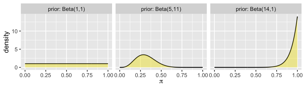
FIGURE 4.1: Three prior models for the proportion of films that pass the Bechdel test.

Placing the greatest prior plausibility on values of \(\pi\) that are less than 0.5, the Beta(5,11) prior reflects the feminist’s understanding that the majority of movies fail the Bechdel test. In contrast, the Beta(14,1) places greater prior plausibility on values of \(\pi\) near 1, and thus matches the optimist’s prior understanding. This leaves the Beta(1,1) or Unif(0,1) prior which, by placing equal plausibility on all values of \(\pi\) between 0 and 1, matches the clueless’s figurative shoulder shrug – the only thing they know is that \(\pi\) is a proportion, and thus is somewhere between 0 and 1.

The three analysts agree to review a sample of \(n\) recent movies and record \(Y\), the number that pass the Bechdel test. Recognizing \(Y\) as the number of “successes” in a fixed number of independent trials, they specify the dependence of \(Y\) on \(\pi\) using a Binomial model. Thus, each analyst has a unique Beta-Binomial model of \(\pi\) with differing prior hyperparameters \(\alpha\) and \(\beta\):

\[\begin{split} Y | \pi & \sim \text{Bin}(n, \pi) \\ \pi & \sim \text{Beta}(\alpha, \beta) \\ \end{split} .\]

By our work in Chapter 3, it follows that each analyst has a unique posterior model of \(\pi\) which depends upon their unique prior (through \(\alpha\) and \(\beta\)) and the common observed data (through \(y\) and \(n\))

\[\begin{equation} \pi | (Y = y) \sim \text{Beta}(\alpha + y, \beta + n - y) . \tag{4.1} \end{equation}\]

If you’re thinking “Can everyone have their own prior?! Is this always going to be so subjective?!” you are asking the right questions! And the questions don’t end there. To what extent might their different priors lead the analysts to three different posterior conclusions about the Bechdel test? How might this depend upon the sample size and outcomes of the movie data they collect? To what extent will the analysts’ posterior understandings evolve as they collect more and more data? Will they ever come to agreement about the representation of women in film?! We will examine these fundamental questions throughout Chapter 4, continuing to build our capacity to think like Bayesians.

• Explore the balanced influence of the prior and data on the posterior. You will see how our choice of prior model, the features of our data, and the delicate balance between them can impact the posterior model.

• Perform sequential Bayesian analysis. You will explore one of the coolest features of Bayesian analysis: how a posterior model evolves as it’s updated with new data.

# Load packages that will be used in this chapter
library(bayesrules)
library(tidyverse)
library(janitor)

4.1 Different priors, different posteriors

Reexamine Figure 4.1 which summarizes the prior models of \(\pi\), the proportion of recent movies that pass the Bechdel test, tuned by the clueless, the feminist, and the optimist. Not only do the differing prior means reflect disagreement about whether \(\pi\) is closer to 0 or 1, the differing levels of prior variability reflect the fact that the analysts have different degrees of certainty in their prior information. Loosely speaking, the more certain the prior information, the smaller the prior variability. The more vague the prior information, the greater the prior variability. The priors of the optimist and the clueless represent these two extremes. With a Beta(14,1) prior which exhibits the smallest variability, the optimist is the most certain in their prior understanding of \(\pi\) (specifically, that almost all movies pass the Bechdel test). We refer to such priors as informative.

Informative prior

An informative prior reflects specific information about the unknown variable with high certainty, i.e., low variability.

With the largest prior variability, the clueless is the least certain about \(\pi\). In fact, their Beta(1,1) prior assigns equal prior plausibility to each value of \(\pi\) between 0 and 1. This type of “shoulder shrug” prior model has an official name: it’s a vague prior.

Vague prior

A vague or diffuse prior reflects little specific information about the unknown variable. A flat prior, which assigns equal prior plausibility to all possible values of the variable, is a special case.

The next natural question to ask is: how will their different priors influence the posterior conclusions of the feminist, the clueless, and the optimist? To answer this question, we need some data. Our analysts decide to review a random sample of \(n = 20\) recent movies using data collected for the FiveThirtyEight article on the Bechdel test.³² The bayesrules package includes a partial version of this dataset, named bechdel. A complete version is provided by the fivethirtyeight R package (Kim, Ismay, and Chunn 2020). Along with the title and year of each movie in this dataset, the binary variable records whether the film passed or failed the Bechdel test:

# Import data
data(bechdel, package = "bayesrules")

# Take a sample of 20 movies
set.seed(84735)
bechdel_20 <- bechdel %>% 
  sample_n(20)

bechdel_20 %>% 
  head(3)
# A tibble: 3 x 3
   year title      binary
  <dbl> <chr>      <chr> 
1  2005 King Kong  FAIL  
2  1983 Flashdance PASS  
3  2013 The Purge  FAIL  

Among the 20 movies in this sample, only 9 (45%) passed the test:

bechdel_20 %>% 
  tabyl(binary) %>% 
  adorn_totals("row")
 binary  n percent
   FAIL 11    0.55
   PASS  9    0.45
  Total 20    1.00

Before going through any formal math, perform the following gut check of how you expect each analyst to react to this data. Answers are discussed below.

The figure below displays our three analysts’ unique priors along with the common scaled likelihood function which reflects the \(Y = 9\) of \(n = 20\) (45%) sampled movies that passed the Bechdel test. Whose posterior do you anticipate will look the most like the scaled likelihood? That is, whose posterior understanding of the Bechdel test pass rate will most agree with the observed 45% rate in the observed data? Whose do you anticipate will look the least like the scaled likelihood?

The three analysts’ posterior models of \(\pi\), which follow from applying (4.1) to their unique prior models and common movie data, are summarized in Table 4.1 and Figure 4.2. For example, the feminist’s posterior parameters are calculated by \(\alpha + y = 5 + 9 = 14\) and \(\beta + n - y = 11 + 20 - 9 = 22\).

TABLE 4.1: The prior and posterior models for \(\pi\), constructed in light of the data that \(Y = 9\) of \(n = 20\) sampled movies pass the Bechdel test.

Analyst	Prior	Posterior
the feminist	Beta(5,11)	Beta(14,22)
the clueless	Beta(1,1)	Beta(10,12)
the optimist	Beta(14,1)	Beta(23,12)

Were your instincts right? Recall that the optimist started with the most insistently optimistic prior about \(\pi\) – their prior model had a high mean with low variability. It’s not very surprising then that their posterior model isn’t as in sync with the data as the other analysts’ posteriors. The dismal data in which only 45% of the 20 sampled movies passed the test wasn’t enough to convince them that there’s a problem in Hollywood – they still think that values of \(\pi\) above 0.5 are the most plausible. At the opposite extreme is the clueless who started with a flat, vague prior model of \(\pi\). Absent any prior information, their posterior model directly reflects the insights gained from the observed movie data. In fact, their posterior is indistinguishable from the scaled likelihood function.

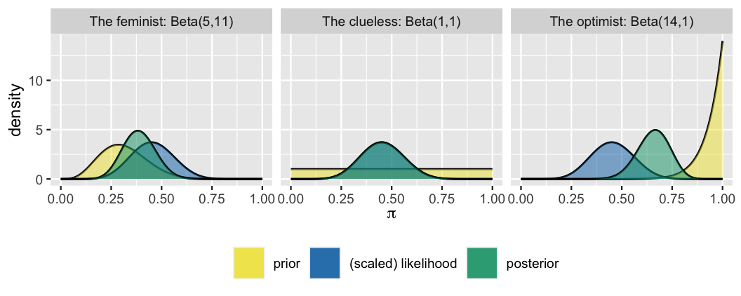
FIGURE 4.2: Posterior models of \(\pi\), constructed in light of the sample in which \(Y = 9\) of \(n = 20\) movies passed the Bechdel.

As a reminder, likelihood functions are not pdfs, and thus typically don’t integrate to 1. As such, the clueless’s actual (unscaled) likelihood is not equivalent to their posterior pdf. We’re merely scaling the likelihood function here for simplifying the visual comparisons between the prior vs data evidence about \(\pi\).

4.2 Different data, different posteriors

If you’re concerned by the fact that our three analysts have differing posterior understandings of \(\pi\), the proportion of recent movies that pass the Bechdel, don’t despair yet. Don’t forget the role that data plays in a Bayesian analysis. To examine these dynamics, consider three new analysts – Morteza, Nadide, and Ursula – who all share the optimistic Beta(14,1) prior for \(\pi\) but each have access to different data. Morteza reviews \(n = 13\) movies from the year 1991, among which \(Y = 6\) (about 46%) pass the Bechdel:

bechdel %>% 
  filter(year == 1991) %>% 
  tabyl(binary) %>% 
  adorn_totals("row")
 binary  n percent
   FAIL  7  0.5385
   PASS  6  0.4615
  Total 13  1.0000

Nadide reviews \(n = 63\) movies from 2000, among which \(Y = 29\) (about 46%) pass the Bechdel:

bechdel %>% 
  filter(year == 2000) %>% 
  tabyl(binary) %>% 
  adorn_totals("row")
 binary  n percent
   FAIL 34  0.5397
   PASS 29  0.4603
  Total 63  1.0000

Finally, Ursula reviews \(n = 99\) movies from 2013, among which \(Y = 46\) (about 46%) pass the Bechdel:

bechdel %>% 
  filter(year == 2013) %>% 
  tabyl(binary) %>% 
  adorn_totals("row")
 binary  n percent
   FAIL 53  0.5354
   PASS 46  0.4646
  Total 99  1.0000

What a coincidence! Though Morteza, Nadide, and Ursula have collected different data, each observes a Bechdel pass rate of roughly 46%. Yet their sample sizes \(n\) differ – Morteza only reviewed 13 movies whereas Ursula reviewed 99. Before doing any formal math, check your intuition about how this different data will lead to different posteriors for the three analysts. Answers are discussed below.

The three analysts’ common prior and unique Binomial likelihood functions (3.12), reflecting their different data, are displayed below. Whose posterior do you anticipate will be most in sync with their data, as visualized by the scaled likelihood? Whose posterior do you anticipate will be the least in sync with their data?

The three analysts’ posterior models of \(\pi\), which follow from applying (4.1) to their common Beta(14,1) prior model and unique movie data, are summarized in Figure 4.3 and Table 4.2. Was your intuition correct? First, notice that the larger the sample size \(n\), the more “insistent” the likelihood function. For example, the likelihood function reflecting the 46% pass rate in Morteza’s small sample of 13 movies is quite wide – his data are relatively plausible for any \(\pi\) between 15% and 75%. In contrast, reflecting the 46% pass rate in a much larger sample of 99 movies, Ursula’s likelihood function is narrow – her data are implausible for \(\pi\) values outside the range from 35% to 55%. In turn, we see that the more insistent the likelihood, the more influence the data holds over the posterior. Morteza remains the least convinced by the low Bechdel pass rate observed in his small sample whereas Ursula is the most convinced. Her early prior optimism evolved into to a posterior understanding that \(\pi\) is likely only between 40% and 55%.

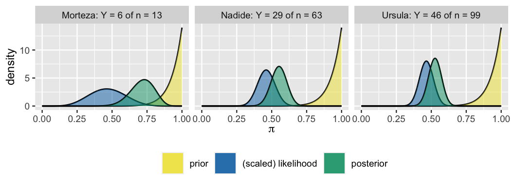
FIGURE 4.3: Posterior models of \(\pi\), constructed from the same prior but different data, are plotted for each analyst.

TABLE 4.2: The prior and posterior models for \(\pi\), constructed in light of a common Beta(14,1) prior and different data.

Analyst	Data	Posterior
Morteza	\(Y = 6\) of \(n = 13\)	Beta(20,8)
Nadide	\(Y = 29\) of \(n = 63\)	Beta(43,35)
Ursula	\(Y = 46\) of \(n = 99\)	Beta(60,54)

4.3 Striking a balance between the prior & data

4.3.1 Connecting observations to concepts

In this chapter, we’ve observed the influence that different priors (Section 4.1) and different data (Section 4.2) can have on our posterior understanding of an unknown variable. However, the posterior is a more nuanced tug-of-war between these two sides. The grid of plots in Figure 4.4 illustrates the balance that the posterior model strikes between the prior and data. Each row corresponds to a unique prior model and each column to a unique set of data.

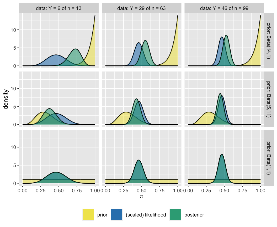
FIGURE 4.4: Posterior models of \(\pi\) constructed under different combinations of prior models and observed data.

Moving from left to right across the grid, the sample size increases from \(n = 13\) to \(n = 99\) movies while preserving the proportion of movies that pass the Bechdel test (\(Y/n \approx 0.46\)). The likelihood’s insistence and, correspondingly, the data’s influence over the posterior increase with sample size \(n\). This also means that the influence of our prior understanding diminishes as we amass new data. Further, the rate at which the posterior balance tips in favor of the data depends upon the prior. Moving from top to bottom across the grid, the priors move from informative (Beta(14,1)) to vague (Beta(1,1)). Naturally, the more informative the prior, the greater its influence on the posterior.

Combining these observations, the last column in the grid delivers a very important Bayesian punchline: no matter the strength of and discrepancies among their prior understanding of \(\pi\), three analysts will come to a common posterior understanding in light of strong data. This observation is a relief. If Bayesian models laughed in the face of more and more data, we’d have a problem.

Play around! To more deeply explore the roles the prior and data play in a posterior analysis, use the plot_beta_binomial() and summarize_beta_binomial() functions in the bayesrules package to visualize and summarize the Beta-Binomial posterior model of \(\pi\) under different combinations of Beta(\(\alpha\), \(\beta\)) prior models and observed data, \(Y\) successes in \(n\) trials:

# Plot the Beta-Binomial model
plot_beta_binomial(alpha = ___, beta = ___, y = ___, n = ___)

# Obtain numerical summaries of the Beta-Binomial model
summarize_beta_binomial(alpha = ___, beta = ___, y = ___, n = ___)

4.3.2 Connecting concepts to theory

The patterns we’ve observed in the posterior balance between the prior and data are intuitive. They’re also supported by an elegant mathematical result. If you’re interested in supporting your intuition with theory, read on. If you’d rather skip the technical details, you can continue on to Section 4.4 without major consequence.

Consider the general Beta-Binomial setting where \(\pi\) is the success rate of some event of interest with a Beta(\(\alpha,\beta\)) prior. Then by (4.1), the posterior model of \(\pi\) upon observing \(Y = y\) successes in \(n\) trials is \(\text{Beta}(\alpha + y, \beta + n - y)\). It follows from (3.11) that the central tendency in our posterior understanding of \(\pi\) can be measured by the posterior mean,

\[E(\pi | Y=y) = \frac{\alpha + y}{\alpha + \beta + n} .\]

And with a little rearranging, we can isolate the influence of the prior and observed data on the posterior mean. The second step in this rearrangement might seem odd, but notice that we’re just multiplying both fractions by 1 (e.g., \(n/n\)).

\[\begin{split} E(\pi | Y=y) & = \frac{\alpha}{\alpha + \beta + n} + \frac{y}{\alpha + \beta + n} \\ & = \frac{\alpha}{\alpha + \beta + n}\cdot\frac{\alpha + \beta}{\alpha + \beta} + \frac{y}{\alpha + \beta + n}\cdot\frac{n}{n} \\ & = \frac{\alpha + \beta}{\alpha + \beta + n}\cdot\frac{\alpha}{\alpha + \beta} + \frac{n}{\alpha + \beta + n}\cdot\frac{y}{n} \\ & = \frac{\alpha + \beta}{\alpha + \beta + n}\cdot E(\pi) + \frac{n}{\alpha + \beta + n}\cdot\frac{y}{n} . \\ \end{split}\]

We’ve now split the posterior mean into two pieces: a piece which depends upon the prior mean \(E(\pi)\) (3.2) and a piece which depends upon the observed success rate in our sample trials, \(y / n\). In fact, the posterior mean is a weighted average of the prior mean and sample success rate, their distinct weights summing to 1:
\[\frac{\alpha + \beta}{\alpha + \beta + n} + \frac{n}{\alpha + \beta + n} = 1 .\]

For example, consider the posterior means for Morteza and Ursula, the settings for which are summarized in Table 4.2. With a shared Beta(14,1) prior for \(\pi\), Morteza and Ursula share a prior mean of \(E(\pi) = 14/15\). Yet their data differs. Morteza observed \(Y = 6\) of \(n = 13\) films pass the Bechdel test, and thus has a posterior mean of

\[\begin{split} E(\pi | Y=6) & = \frac{14 + 1}{14 + 1 + 13} \cdot E(\pi) + \frac{13}{14 + 1 + 13}\cdot\frac{y}{n} \\ & = 0.5357 \cdot \frac{14}{15} + 0.4643 \cdot \frac{6}{13} \\ & = 0.7143 . \\ \end{split}\]

Ursula observed \(Y = 46\) of \(n = 99\) films pass the Bechdel test, and thus has a posterior mean of

\[\begin{split} E(\pi | Y=46) & = \frac{14 + 1}{14 + 1 + 99} \cdot E(\pi) + \frac{99}{14 + 1 + 99}\cdot\frac{y}{n} \\ & = 0.1316 \cdot \frac{14}{15} + 0.8684 \cdot \frac{46}{99} \\ & = 0.5263 . \\ \end{split}\]

Again, though Morteza and Ursula have a common prior mean for \(\pi\) and observed similar Bechdel pass rates of roughly 46%, their posterior means differ due to their differing sample sizes \(n\). Since Morteza observed only \(n = 13\) films, his posterior mean put slightly more weight on the prior mean than on the observed Bechdel pass rate in his sample: 0.5357 vs 0.4643. In contrast, since Ursula observed a relatively large number of \(n = 99\) films, her posterior mean put much less weight on the prior mean than on the observed Bechdel pass rate in her sample: 0.1316 vs 0.8684.

The implications of these results are mathemagical. In general, consider what happens to the posterior mean as we collect more and more data. As sample size \(n\) increases, the weight (hence influence) of the Beta(\(\alpha,\beta\)) prior model approaches 0,

\[\frac{\alpha + \beta}{\alpha + \beta + n} \to 0 \;\; \text{ as } n \to \infty,\]

while the weight (hence influence) of the data approaches 1,

\[\frac{n}{\alpha + \beta + n} \to 1 \;\; \text{ as } n \to \infty.\]

Thus, the more data we have, the more the posterior mean will drift toward the trends exhibited in the data as opposed to the prior: as \(n \to \infty\)

\[E(\pi | Y=y) = \frac{\alpha + \beta}{\alpha + \beta + n}\cdot E(\pi) + \frac{n}{\alpha + \beta + n}\cdot\frac{y}{n} \;\;\; \to \;\;\; \frac{y}{n} .\]

The rate at which this drift occurs depends upon whether the prior tuning (i.e., \(\alpha\) and \(\beta\)) is informative or vague. Thus, these mathematical results support the observations we made about the posterior’s balance between the prior and data in Figure 4.4. And that’s not all! In the exercises, you will show that we can write the posterior mode as the weighted average of the prior mode and observed sample success rate:

\[\text{Mode}(\pi | Y=y) = \frac{\alpha + \beta - 2}{\alpha + \beta + n - 2} \cdot\text{Mode}(\pi) + \frac{n}{\alpha + \beta + n - 2} \cdot\frac{y}{n} .\]

4.4 Sequential analysis: Evolving with data

In our discussions above, we examined the increasing influence of the data and diminishing influence of the prior on the posterior as more and more data come in. Consider the nuances of this concept. The phrase “as more and more data come in” evokes the idea that data collection, and thus the evolution in our posterior understanding, happens incrementally. For example, scientists’ understanding of climate change has evolved over the span of decades as they gain new information. Presidential candidates’ understanding of their chances of winning an election evolve over months as new poll results become available. Providing a formal framework for this evolution is one of the most powerful features of Bayesian statistics!

Let’s revisit Milgram’s behavioral study of obedience from Section 3.6. In this setting, \(\pi\) represents the proportion of people that will obey authority even if it means bringing harm to others. In Milgram’s study, obeying authority meant delivering a severe electric shock to another participant (which, in fact, was a ruse). Prior to Milgram’s experiments, our fictional psychologist expected that few people would obey authority in the face of harming another: \(\pi \sim \text{Beta}(1,10)\). They later observed that 26 of 40 study participants inflicted what they understood to be a severe shock.

Now, suppose that the psychologist collected this data incrementally, day by day, over a three-day period. Each day, they evaluated \(n\) subjects and recorded \(Y\), the number that delivered the most severe shock (thus \(Y | \pi \sim \text{Bin}(n,\pi)\)). Among the \(n = 10\) day-one participants, only \(Y = 1\) delivered the most severe shock. Thus, by the end of day one, the psychologist’s understanding of \(\pi\) had already evolved. It follows from (4.1) that³³

\[\pi | (Y = 1) \sim \text{Beta}(2,19) .\]

Day two was much busier and the results grimmer: among \(n = 20\) participants, \(Y = 17\) delivered the most severe shock. Thus, by the end of day two, the psychologist’s understanding of \(\pi\) had again evolved – \(\pi\) was likely larger than they had expected.

What was the psychologist’s posterior of \(\pi\) at the end of day two?

1. Beta(19,22)
2. Beta(18,13)

If your answer is “a,” you are correct! On day two, the psychologist didn’t simply forget what happened on day one and start afresh with the original Beta(1,10) prior. Rather, what they had learned by the end of day one, expressed by the Beta(2,19) posterior, provided a prior starting point on day two. Thus, by (4.1), the posterior model of \(\pi\) at the end of day two is Beta(19,22).³⁴ On day three, \(Y = 8\) of \(n = 10\) participants delivered the most severe shock, and thus their model of \(\pi\) evolved from a Beta(19,22) prior to a Beta(27,24) posterior.³⁵ The complete evolution from the psychologist’s original Beta(1,10) prior to their Beta(27,24) posterior at the end of the three-day study is summarized in Table 4.3. Figure 4.5 displays this evolution in pictures, including the psychologist’s big leap from day one to day two upon observing so many study participants deliver the most severe shock (17 of 20).

TABLE 4.3: A sequential Bayesian analysis of Milgram’s data.

Day	Data	Model
0	NA	Beta(1,10)
1	Y = 1 of n = 10	Beta(2,19)
2	Y = 17 of n = 20	Beta(19,22)
3	Y = 8 of n = 10	Beta(27,24)

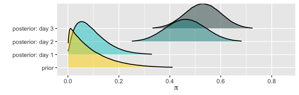
FIGURE 4.5: The sequential analysis of Milgram’s data as summarized by Table 4.3.

The process we’ve just taken, incrementally updating the psychologist’s posterior model of \(\pi\), is referred to more generally as a sequential Bayesian analysis or Bayesian learning.

Sequential Bayesian analysis (aka Bayesian learning)

In a sequential Bayesian analysis, a posterior model is updated incrementally as more data come in. With each new piece of data, the previous posterior model reflecting our understanding prior to observing this data becomes the new prior model.

The ability to evolve as new data come in is one of the most powerful features of the Bayesian framework. These types of sequential analyses also uphold two fundamental and common sensical properties. First, the final posterior model is data order invariant, i.e., it isn’t impacted by the order in which we observe the data. For example, suppose that the psychologist had observed Milgram’s study data in the reverse order: \(Y = 8\) of \(n = 10\) on day one, \(Y = 17\) of \(n = 20\) on day two, and \(Y = 1\) of \(n = 10\) on day three. The resulting evolution in their understanding of \(\pi\) is summarized by Table 4.4 and Figure 4.6. In comparison to their analysis of the reverse data collection (Table 4.3), the psychologist’s evolving understanding of \(\pi\) takes a different path. However, it still ends up in the same place – the Beta(27,24) posterior. These differing evolutions are highlighted by comparing Figure 4.6 to Figure 4.5.

TABLE 4.4: A sequential Bayesian analysis of Milgram’s data, reversing the order in which the data was observed.

Day	Data	Model
0	NA	Beta(1,10)
1	Y = 8 of n = 10	Beta(9,12)
2	Y = 17 of n = 20	Beta(26,15)
3	Y = 1 of n = 10	Beta(27,24)

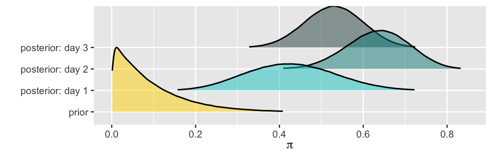
FIGURE 4.6: The sequential analysis of Milgram’s data as summarized by Table 4.4.

The second fundamental feature of a sequential analysis is that the final posterior only depends upon the cumulative data. For example, in the combined three days of Milgram’s experiment, there were \(n = 10 + 20 + 10 = 40\) participants among whom \(Y = 1 + 17 + 8 = 26\) delivered the most severe shock. In Section 3.6, we evaluated this data all at once, not incrementally. In doing so, we jumped straight from the psychologist’s original Beta(1,10) prior model to the Beta(27,24) posterior model of \(\pi\). That is, whether we evaluate the data incrementally or all in one go, we’ll end up at the same place.

4.5 Proving data order invariance

In the previous section, you saw evidence of data order invariance in action. Here we’ll prove that this feature is enjoyed by all Bayesian models. This section is fun but not a deal breaker to your future work.

Data order invariance

Let \(\theta\) be any parameter of interest with prior pdf \(f(\theta)\). Then a sequential analysis in which we first observe a data point \(y_1\) and then a second data point \(y_2\) will produce the same posterior model of \(\theta\) as if we first observe \(y_2\) and then \(y_1\):

\[f(\theta | y_1,y_2) = f(\theta|y_2,y_1).\]

Similarly, the posterior model is invariant to whether we observe the data all at once or sequentially.

To prove the data order invariance property, let’s first specify the structure of posterior pdf \(f(\theta | y_1,y_2)\) which evolves by sequentially observing data \(y_1\) followed by \(y_2\). In step one of this evolution, we construct the posterior pdf from our original prior pdf, \(f(\theta)\), and the likelihood function of \(\theta\) given the first data point \(y_1\), \(L(\theta|y_1)\):

\[f(\theta|y_1) = \frac{\text{prior}\cdot \text{likelihood}}{\text{normalizing constant}} = \frac{f(\theta)L(\theta|y_1)}{f(y_1)} .\]

In step two, we update our model in light of observing new data \(y_2\). In doing so, don’t forget that we start from the prior model specified by \(f(\theta|y_1)\), and thus

\[f(\theta|y_2) = \frac{\frac{f(\theta)L(\theta|y_1)}{f(y_1)}L(\theta|y_2)}{f(y_2)} = \frac{f(\theta)L(\theta|y_1)L(\theta|y_2)}{f(y_1)f(y_2)} . \]

Similarly, observing the data in the opposite order, \(y_2\) and then \(y_1\), would produce the equivalent posterior:

\[f(\theta|y_2,y_1) = \frac{f(\theta)L(\theta|y_2)L(\theta|y_1)}{f(y_2)f(y_1)} . \]

Finally, not only does the order of the data not influence the ultimate posterior model of \(\theta\), it doesn’t matter whether we observe the data all at once or sequentially. To this end, suppose we start with the original \(f(\theta)\) prior and observe data \((y_1,y_2)\) together, not sequentially. Further, assume that these data points are unconditionally and conditionally independent, and thus

\[f(y_1,y_2) = f(y_1)f(y_2) \;\; \text{ and } \;\; f(y_1,y_2 | \theta) = f(y_1|\theta)f(y_2|\theta) .\]

Then the posterior pdf resulting from this “data dump” is equivalent to that resulting from the sequential analyses above:

\[\begin{split} f(\theta|y_1,y_2) & = \frac{f(\theta)L(\theta|y_1,y_2)}{f(y_1,y_2)} \\ & = \frac{f(\theta)f(y_1,y_2|\theta)}{f(y_1)f(y_2)} \\ & = \frac{f(\theta)L(\theta|y_1)L(\theta|y_2)}{f(y_1)f(y_2)} . \\ \end{split}\]

4.6 Don’t be stubborn

Chapter 4 has highlighted some of the most compelling aspects of the Bayesian philosophy – it provides the framework and flexibility for our understanding to evolve over time. One of the only ways to lose this Bayesian benefit is by starting with an extremely stubborn prior model. A model so stubborn that it assigns a prior probability of zero to certain parameter values. Consider an example within the Milgram study setting where \(\pi\) is the proportion of people that will obey authority even if it means bringing harm to others. Suppose that a certain researcher has a stubborn belief in the good of humanity, insisting that \(\pi\) is equally likely to be anywhere between 0 and 0.25, and surely doesn’t exceed 0.25. They express this prior understanding through a Uniform model on 0 to 0.25,

\[\pi \sim \text{Unif}(0,0.25)\]

with pdf \(f(\pi)\) exhibited in Figure 4.7 and specified by

\[f(\pi) = 4 \; \text{ for } \pi \in [0, 0.25] .\]

Now, suppose this researcher was told that the first \(Y = 8\) of \(n = 10\) participants delivered the shock. This 80% figure runs counter to the stubborn researcher’s belief. Check your intuition about how the researcher will update their posterior in light of this data.

The stubborn researcher’s prior pdf and likelihood function are illustrated in each plot of Figure 4.7. Which plot accurately depicts the researcher’s corresponding posterior?

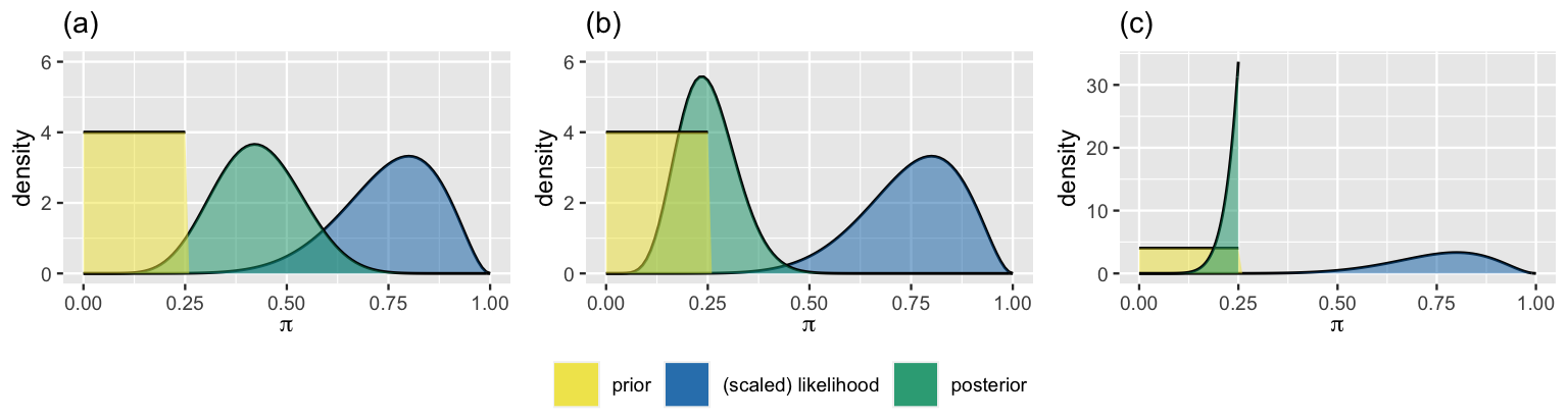
FIGURE 4.7: The stubborn researcher’s prior and likelihood, with three potential corresponding posterior models.

As odd as it might seem, the posterior model in plot (c) corresponds to the stubborn researcher’s updated understanding of \(\pi\) in light of the observed data. A posterior model is defined on the same values for which the prior model is defined. That is, the support of the posterior model is inherited from the support of the prior model. Since the psychologist’s prior model assigns zero probability to any value of \(\pi\) past 0.25, their posterior model must also assign zero probability to any value in that range. Mathematically, the posterior pdf \(f(\pi | y=8) = 0\) for any \(\pi \notin [0,0.25]\) and, for any \(\pi \in [0, 0.25]\),

\[\begin{split} f(\pi | y=8) & \propto f(\pi)L(\pi | y=8) \\ & = 4 \cdot \left(\!\begin{array}{c} 10 \\ 8 \end{array}\!\right) \ \pi^{8} (1-\pi)^{2} \\ & \propto \pi^{8} (1-\pi)^{2}. \\ \end{split}\]

The implications of this math are huge. No matter how much counterevidence the stubborn researcher collects, their posterior will never budge beyond the 0.25 cap, not even if they collect data on a billion subjects. Luckily, we have some good news for you: this Bayesian bummer is completely preventable.

Hot tip: How to avoid a regrettable prior model

Let \(\pi\) be some parameter of interest. No matter how much prior information you think you have about \(\pi\) or how informative you want to make your prior, be sure to assign non-0 plausibility to every possible value of \(\pi\), even if this plausibility is near 0. For example, if \(\pi\) is a proportion which can technically range from 0 to 1, then your prior model should also be defined across this continuum.

4.7 A note on subjectivity

In Chapter 1, we alluded to a common critique about Bayesian statistics – it’s too subjective. Specifically, some worry that “subjectively” tuning a prior model allows a Bayesian analyst to come to any conclusion that they want to. We can more rigorously push back against this critique in light of what we’ve learned in Chapter 4. Before we do, reconnect to and expand upon some concepts that you’ve explored throughout the book.

For each statement below, indicate whether the statement is true or false. Provide your reasoning.

1. All prior choices are informative.
2. There may be good reasons for having an informative prior.
3. Any prior choice can be overcome by enough data.
4. The frequentist paradigm is totally objective.

Answers are provided in the footnotes.³⁶ Consider the main points. Throughout Chapter 4, you’ve confirmed that a Bayesian can indeed build a prior based on “subjective” experience. Very seldom is this a bad thing, and quite often it’s a great thing! In the best-case scenarios, a subjective prior can reflect a wealth of past experiences that should be incorporated into our analysis – it would be unfortunate not to. Even if a subjective prior runs counter to actual observed evidence, its influence over the posterior fades away as this evidence piles up. We’ve seen one worst-case scenario exception. And it was preventable. If a subjective prior is stubborn enough to assign zero probability on a possible parameter value, no amount of counterevidence will be enough to budge it.

Finally, though we encourage you to be critical in your application of Bayesian methods, please don’t worry about them being any more subjective than frequentist methods. No human is capable of removing all subjectivity from an analysis. The life experiences and knowledge we carry with us inform everything from what research questions we ask to what data we collect. It’s important to consider the potential implications of this subjectivity in both Bayesian and frequentist analyses.

4.8 Chapter summary

In Chapter 4 we explored the balance that a posterior model strikes between a prior model and the data. In general, we saw the following trends:

• Prior influence
  The less vague and more informative the prior, i.e., the greater our prior certainty, the more influence the prior has over the posterior.

• Data influence
  The more data we have, the more influence the data has over the posterior. Thus, if they have ample data, two researchers with different priors will have similar posteriors.

Further, we saw that in a sequential Bayesian analysis, we incrementally update our posterior model as more and more data come in. The final destination of this posterior is not impacted by the order in which we observe this data (i.e., the posterior is data order invariant) or whether we observe the data in one big dump or incrementally.

4.9 Exercises

4.9.1 Review exercises

Exercise 4.1 (Match the prior to the description) Five different prior models for \(\pi\) are listed below. Label each with one of these descriptors: somewhat favoring \(\pi<0.5\), strongly favoring \(\pi<0.5\), centering \(\pi\) on 0.5, somewhat favoring \(\pi>0.5\), strongly favoring \(\pi>0.5\).

1. Beta(1.8,1.8)
2. Beta(3,2)
3. Beta(1,10)
4. Beta(1,3)
5. Beta(17,2)

Exercise 4.2 (Match the plot to the code) Which arguments to the plot_beta_binomial() function generated the plot below?

1. alpha = 2, beta = 2, y = 8, n = 11
2. alpha = 2, beta = 2, y = 3, n = 11
3. alpha = 3, beta = 8, y = 2, n = 6
4. alpha = 3, beta = 8, y = 4, n = 6
5. alpha = 3, beta = 8, y = 2, n = 4
6. alpha = 8, beta = 3, y = 2, n = 4

Exercise 4.3 (Choice of prior: gingko tree leaf drop) A ginkgo tree can grow into a majestic monument to the wonders of the natural world. One of the most notable things about ginkgo trees is that they shed all of their leaves at the same time, usually after the first frost. Randi thinks that the ginkgo tree in her local arboretum will drop all of its leaves next Monday. She asks 5 of her friends what they think about the probability (\(\pi\)) that this will happen. Identify some reasonable Beta priors to convey each of these beliefs.

1. Ben says that it is really unlikely.
2. Albert says that he is quite unsure and hates trees. He has no idea.
3. Katie gives it some thought and, based on what happened last year, thinks that there is a very high chance.
4. Daryl thinks that there is a decent chance, but he is somewhat unsure.
5. Scott thinks it probably won’t happen, but he’s somewhat unsure.

4.9.2 Practice: Different priors, different posteriors

For all exercises in this section, consider the following story. The local ice cream shop is open until it runs out of ice cream for the day. It’s 2 p.m. and Chad wants to pick up an ice cream cone. He asks his coworkers about the chance (\(\pi\)) that the shop is still open. Their Beta priors for \(\pi\) are below:

coworker	prior
Kimya	Beta(1, 2)
Fernando	Beta(0.5, 1)
Ciara	Beta(3, 10)
Taylor	Beta(2, 0.1)

Exercise 4.4 (Choice of prior) Visualize and summarize (in words) each coworker’s prior understanding of Chad’s chances to satisfy his ice cream craving.

Exercise 4.5 (Simulating the posterior) Chad peruses the shop’s website. On 3 of the past 7 days, they were still open at 2 p.m.. Complete the following for each of Chad’s coworkers:

• simulate their posterior model;
• create a histogram for the simulated posterior; and
• use the simulation to approximate the posterior mean value of \(\pi\).

Exercise 4.6 (Identifying the posterior) Complete the following for each of Chad’s coworkers:

• identify the exact posterior model of \(\pi\);
• calculate the exact posterior mean of \(\pi\); and
• compare these to the simulation results in the previous exercise.

4.9.3 Practice: Balancing the data & prior

Exercise 4.7 (What dominates the posterior?) In each situation below you will be given a Beta prior for \(\pi\) and some Binomial trial data. For each scenario, identify which of the following is true: the prior has more influence on the posterior, the data has more influence on the posterior, or the posterior is an equal compromise between the data and the prior.

1. Prior: \(\pi \sim \text{Beta}(1, 4)\), data: \(Y = 8\) successes in \(n = 10\) trials
2. Prior: \(\pi \sim \text{Beta}(20, 3)\), data: \(Y = 0\) successes in \(n = 1\) trial
3. Prior: \(\pi \sim \text{Beta}(4, 2)\), data: \(Y = 1\) success in \(n = 3\) trials
4. Prior: \(\pi \sim \text{Beta}(3, 10)\), data: \(Y = 10\) successes in \(n = 13\) trials
5. Prior: \(\pi \sim \text{Beta}(20, 2)\), data: \(Y = 10\) successes in \(n = 200\) trials

Exercise 4.8 (Visualizing the evolution) For each scenario in Exercise 4.7, plot and compare the prior pdf, scaled likelihood function, and posterior pdf for \(\pi\).

Exercise 4.9 (Different data: more or less sure) Let \(\pi\) denote the proportion of people that prefer dogs to cats. Suppose you express your prior understanding of \(\pi\) by a Beta(7, 2) model.

1. According to your prior, what are reasonable values for \(\pi\)?
2. If you observe a survey in which \(Y = 19\) of \(n = 20\) people prefer dogs, how would that change your understanding of \(\pi\)? Comment on both the evolution in your mean understanding and your level of certainty about \(\pi\).
3. If instead, you observe that only \(Y = 1\) of \(n = 20\) people prefer dogs, how would that change your understanding about \(\pi\)?
4. If instead, you observe that \(Y = 10\) of \(n = 20\) people prefer dogs, how would that change your understanding about \(\pi\)?

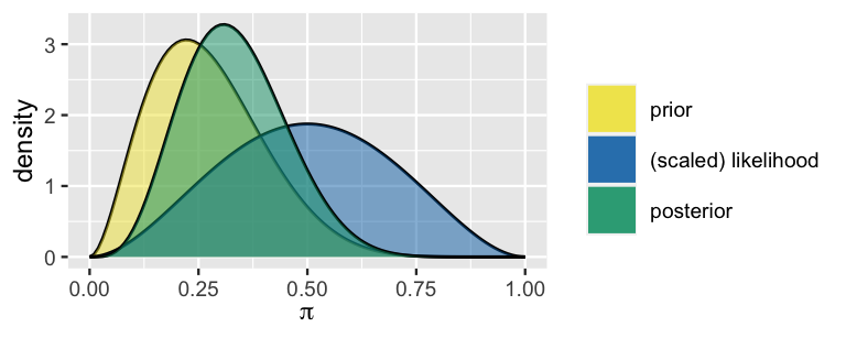
Exercise 4.10 (What was the data?) In each situation below we give you a Beta prior and a Beta posterior. Further, we tell you that the data is Binomial, but we don’t tell you the observed number of trials \(n\) or successes \(y\) in those trials. For each situation, identify \(n\) and \(y\), and then utilize plot_beta_binomial() to sketch the prior pdf, scaled likelihood function, and posterior pdf.

1. Prior: Beta(0.5, 0.5), Posterior: Beta(8.5, 2.5)
2. Prior: Beta(0.5, 0.5), Posterior: Beta(3.5, 10.5)
3. Prior: Beta(10, 1), Posterior: Beta(12, 15)
4. Prior: Beta(8, 3), Posterior: Beta(15, 6)
5. Prior: Beta(2, 2), Posterior: Beta(5, 5)
6. Prior: Beta(1, 1), Posterior: Beta(30, 3)

Exercise 4.11 (Different data, uninformative prior) In each situation below we have the same prior on the probability of a success, \(\pi \sim \text{Beta}(1, 1)\), but different data. Identify the corresponding posterior model and utilize plot_beta_binomial() to sketch the prior pdf, likelihood function, and posterior pdf.

1. \(Y = 10\) in \(n = 13\) trials
2. \(Y = 0\) in \(n = 1\) trial
3. \(Y = 100\) in \(n = 130\) trials
4. \(Y = 20\) in \(n = 120\) trials
5. \(Y = 234\) in \(n = 468\) trials

Exercise 4.12 (Different data, informative prior) Repeat Exercise 4.11, this time assuming a \(\pi \sim \text{Beta}(10, 2)\) prior.

Exercise 4.13 (Bayesian bummer) Bayesian methods are great! But, like anything, we can screw it up. Suppose a politician specifies their prior understanding about their approval rating, \(\pi\), by: \(\pi \sim \text{Unif}(0.5,1)\) with pdf \(f(\pi) = 2\) when \(0.5 \le \pi < 1\), and \(f(\pi) = 0\) when \(0 < \pi < 0.5\).

1. Sketch the prior pdf (by hand).
2. Describe the politician’s prior understanding of \(\pi\).
3. The politician’s aides show them a poll in which 0 of 100 people approve of their job performance. Construct a formula for and sketch the politician’s posterior pdf of \(\pi\).
4. Describe the politician’s posterior understanding of \(\pi\). Use this to explain the mistake the politician made in specifying their prior.

Exercise 4.14 (Challenge: posterior mode)

1. In the Beta-Binomial setting, show that we can write the posterior mode of \(\pi\) as the weighted average of the prior mode and observed sample success rate:

   \[\text{Mode}(\pi | Y=y) = \frac{\alpha + \beta - 2}{\alpha + \beta + n - 2} \cdot\text{Mode}(\pi) + \frac{n}{\alpha + \beta + n - 2} \cdot\frac{y}{n} .\]

2. To what value does the posterior mode converge as our sample size \(n\) increases? Support your answer with evidence.

4.9.4 Practice: Sequentiality

Exercise 4.15 (One at a time) Let \(\pi\) be the probability of success for some event of interest. You place a Beta(2, 3) prior on \(\pi\), and are really impatient. Sequentially update your posterior for \(\pi\) with each new observation below.

1. First observation: Success
2. Second observation: Success
3. Third observation: Failure
4. Fourth observation: Success

Exercise 4.16 (Five at a time) Let \(\pi\) be the probability of success for some event of interest. You place a Beta(2, 3) prior on \(\pi\), and are impatient, but you have been working on that aspect of your personality. So you sequentially update your posterior model of \(\pi\) after every five (!) new observations. For each set of five new observations, report the updated posterior model for \(\pi\).

1. First set of observations: 3 successes
2. Second set of observations: 1 success
3. Third set of observations: 1 success
4. Fourth set of observations: 2 successes

Exercise 4.17 (Different data, different posteriors) A shoe company develops a new internet ad for their latest sneaker. Three employees share the same Beta(4, 3) prior model for \(\pi\), the probability that a user will click on the ad when shown. However, the employees run three different studies, thus each has access to different data. The first employee tests the ad on 1 person – they do not click on the ad. The second tests 10 people, 3 of whom click on the ad. The third tests 100 people, 20 of whom click on the ad.

1. Sketch the prior pdf using plot_beta(). Describe the employees’ prior understanding of the chance that a user will click on the ad.
2. Specify the unique posterior model of \(\pi\) for each of the three employees. We encourage you to construct these posteriors “from scratch,” i.e., without relying on the Beta-Binomial posterior formula.
3. Plot the prior pdf, likelihood function, and posterior pdf for each employee.
4. Summarize and compare the employees’ posterior models of \(\pi\).

Exercise 4.18 (A sequential employee) The shoe company described in Exercise 4.17 brings in a fourth employee. They start with the same Beta(4, 3) prior for \(\pi\) as the first three employees but, not wanting to re-create work, don’t collect their own data. Instead, in their first day on the job, the new employee convinces the first employee to share their data. On the second day they get access to the second employee’s data and on the third day they get access to the third employee’s data.

1. Suppose the new employee updates their posterior model of \(\pi\) at the end of each day. What’s their posterior at the end of day one? At the end of day two? At the end of day three?
2. Sketch the new employee’s prior and three (sequential) posteriors. In words, describe how their understanding of \(\pi\) evolved over their first three days on the job.
3. Suppose instead that the new employee didn’t update their posterior until the end of their third day on the job, after they’d gotten data from all three of the other employees. Specify their posterior model of \(\pi\) and compare this to the day three posterior from part (a).

Exercise 4.19 (Bechdel test) In this exercise we’ll analyze \(\pi\), the proportion of films that pass the Bechdel test, using the bechdel data. For each scenario below, specify the posterior model of \(\pi\), and calculate the posterior mean and mode.

1. John has a flat Beta(1, 1) prior and analyzes movies from the year 1980.
2. The next day, John analyzes movies from the year 1990, while building off their analysis from the previous day.
3. The third day, John analyzes movies from the year 2000, while again building off of their analyses from the previous two days.
4. Jenna also starts her analysis with a Beta(1, 1) prior, but analyzes movies from 1980, 1990, 2000 all on day one.

Exercise 4.20 (Bayesian and frequentist: sequential edition) You learned in this chapter that we can use Bayes to sequentially update our understanding of a parameter of interest. How is this different from what the frequentist approach would be? How is it similar?

References

Bechdel, Alison. 1986. Dykes to Watch Out for. Firebrand Books.

Kim, Albert Y., Chester Ismay, and Jennifer Chunn. 2020. Fivethirtyeight: Data and Code Behind the Stories and Interactives at FiveThirtyEight. https://CRAN.R-project.org/package=fivethirtyeight.

---

31. Answer: Beta(1,1) = clueless prior. Beta(5,11) = feminist prior. Beta(14,1) = optimist prior.↩︎

32. https://fivethirtyeight.com/features/the-dollar-and-cents-case-against-hollywoods-exclusion-of-women/↩︎

33. The posterior parameters are calculated by \(\alpha + y = 1 + 1\) and \(\beta + n - y = 10 + 10 - 1\).↩︎

34. The posterior parameters are calculated by \(\alpha + y = 2 + 17\) and \(\beta + n - y = 19 + 20 - 17\).↩︎

35. The posterior parameters are calculated by \(\alpha + y = 19 + 8\) and \(\beta + n - y = 22 + 10 - 8\).↩︎

36. 1. False. Vague priors are typically uninformative. 2. True. We might have ample previous data or expertise from which to build our prior. 3. False. If you assign zero prior probability to a potential parameter value, no amount of data can change that! 4. False. Subjectivity always creeps in to both frequentist and Bayesian analyses. With the Bayesian paradigm, we can at least name and quantify aspects of this subjectivity.↩︎