Chapter 7 MCMC under the Hood

In Chapter 6, we discussed the need for MCMC posterior simulation in advanced Bayesian analyses and how to achieve these ends using the rstan package. You now have everything you need to analyze more sophisticated Bayesian models in Unit 3 and beyond. Mainly, you can drive from point a to point b without a working understanding of the engine. However, whether now or later, it will be beneficial to your deeper understanding of Bayesian methodology (and fun) to learn about how MCMC methods actually work. We’ll take a peak under the hood in Chapter 7. If learning about computation isn’t your thing at this particular point in time, you’ll still be able to do everything that comes after this chapter. You do you.

Bayesian MCMC simulation is a rich field, spanning various algorithms that share a common goal: approximate the posterior model. For example, the rstan package utilized throughout this book employs a Hamiltonian Monte Carlo algorithm. The alternative rjags package for Bayesian modeling employs a Gibbs sampling algorithm. Though the details differ, both algorithms are variations on the fundamental Metropolis-Hastings algorithm. Thus, instead of studying all variations, which would require a book itself, we’ll focus our attention on the Metropolis-Hastings in Chapter 7. You will both build intuition for this algorithm and learn how to implement it, from scratch, in R. Though this implementation will require computer programming skills that are otherwise outside the scope of this book (e.g., writing functions and for loops), we’ll keep the focus on the concepts so that all can follow along.

# Load packages you'll need for this chapter
library(tidyverse)

• Build a strong conceptual understanding of how Markov chain algorithms work.
• Explore the foundational Metropolis-Hastings algorithm.
• Implement the Metropolis-Hastings algorithm in the Normal-Normal and Beta-Binomial settings.

7.1 The big idea

Consider the following Normal-Normal model with numerical outcome \(Y\) that varies Normally around an unknown mean \(\mu\) with a standard deviation of 0.75:

\[\begin{equation} \begin{split} Y|\mu & \sim \text{N}(\mu, 0.75^2) \\ \mu & \sim \text{N}(0, 1^2) \\ \end{split} \tag{7.1} \end{equation}\]

The corresponding likelihood function \(L(\mu|y)\) and prior pdf \(f(\mu)\) for \(y \in (-\infty, \infty)\) and \(\mu \in (-\infty, \infty)\) are:

\[\begin{equation} L(\mu|y) = \frac{1}{\sqrt{2\pi \cdot 0.75^2}} \exp\bigg[{-\frac{(y-\mu)^2}{2 \cdot 0.75^2}}\bigg] \;\;\;\;\; \text{ and } \;\;\;\;\; f(\mu) = \frac{1}{\sqrt{2\pi}} \exp\bigg[{-\frac{\mu^2}{2}}\bigg] . \tag{7.2} \end{equation}\]

Suppose we observe an outcome \(Y = 6.25\). Then by our Normal-Normal work in Chapter 5 (5.15), the posterior model of \(\mu\) is Normal with mean 4 and standard deviation 0.6:

\[\mu | (Y = 6.25) \sim \text{N}(4, 0.6^2) .\]

As we saw in Chapter 6, if we weren’t able to specify this posterior model of \(\mu\) (just pretend), we could approximate it using MCMC simulation. To get a sense for how this works, consider the results of a potential \(N = 5000\) iteration MCMC simulation (Figure 7.1). It helps to think of the illustrated Markov chain \(\left\lbrace \mu^{(1)}, \mu^{(2)}, \ldots, \mu^{(N)} \right\rbrace\) as a tour around the range of posterior plausible values of \(\mu\) and yourself as the tour manager. The trace plot (left) illustrates the tour route or sequence of tour stops, \(\mu^{(i)}\). The histogram (right) illustrates the relative amount of time you spent in each \(\mu\) region throughout the tour.

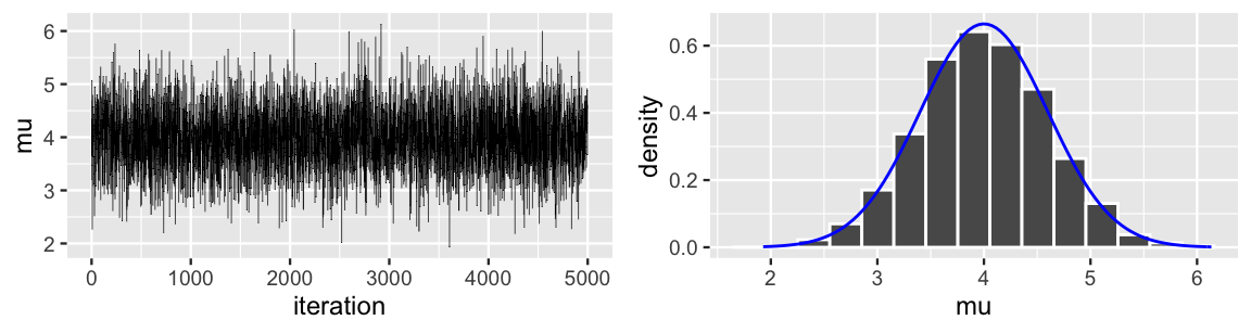
FIGURE 7.1: A trace plot (left) and histogram (right) of a 5,000 iteration MCMC simulation of the \(N(4, 0.6^2)\) posterior. The posterior pdf is superimposed in blue (right).

As tour manager, it’s your job to ensure that the density of tour stops in each \(\mu\) region is proportional to its posterior plausibility. That is, the chain should spend more time touring values of \(\mu\) between 2 and 6, where the Normal posterior pdf is greatest, and less time visiting \(\mu\) values less than 2 or greater than 6, where the posterior drops off. This consideration is crucial to producing a collection of tour stops that accurately approximate the posterior, as does the tour here (Figure 7.1 right).

As tour manager, you can automate the tour route using the Metropolis-Hastings algorithm. This algorithm iterates through a two-step process. Assuming the Markov chain is at location \(\mu^{(i)} = \mu\) at iteration or “tour stop” \(i\), the next tour stop \(\mu^{(i + 1)}\) is selected as follows:

• Step 1: Propose a random location, \(\mu'\), for the next tour stop.
• Step 2: Decide whether to go to the proposed location (\(\mu^{(i+1)} = \mu'\)) or to stay at the current location for another iteration (\(\mu^{(i+1)} = \mu\)).

This might seem easy. For example, if there were no constraints on your tour plan, you could simply draw proposed tour stops \(\mu'\) from the \(\text{N}(4, 0.6^2)\) posterior pdf \(f(\mu' | y = 6.25)\) (Step 1) and then go there (Step 2). This special case of the Metropolis-Hastings algorithm has a special name – Monte Carlo.

Monte Carlo algorithm

To construct an independent Monte Carlo sample directly from posterior pdf \(f(\mu|y)\), \(\left\lbrace \mu^{(1)}, \mu^{(2)}, ..., \mu^{(N)}\right\rbrace\), select each tour stop \(\mu^{(i)} = \mu\) as follows:

• Step 1: Propose a location.
  Draw a location \(\mu\) from the posterior model with pdf \(f(\mu | y)\).
  
• Step 2: Go there.

The Monte Carlo algorithm is so convenient! We can implement this algorithm by simply using rnorm() to sample directly from the \(N(4,0.6^2)\) posterior. The result is a nice independent sample from the posterior which, in turn, produces an accurate posterior approximation:

set.seed(84375)
mc_tour <- data.frame(mu = rnorm(5000, mean = 4, sd = 0.6))
ggplot(mc_tour, aes(x = mu)) + 
  geom_histogram(aes(y = ..density..), color = "white", bins = 15) + 
  stat_function(fun = dnorm, args = list(4, 0.6), color = "blue")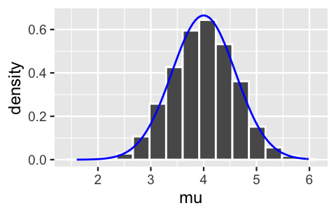

FIGURE 7.2: A histogram of a Monte Carlo sample from the posterior pdf of \(\mu\). The actual pdf is superimposed in blue.

BUT there’s a glitch. Remember that we only need MCMC to approximate a Bayesian posterior when that posterior is too complicated to specify. And if a posterior is too complicated to specify, it’s typically too complicated to directly sample or draw from as we did in our Monte Carlo tour above. This is where the more general Metropolis-Hastings MCMC algorithm comes in. Metropolis-Hastings relies on the fact that, even if we don’t know the posterior model, we do know that the posterior pdf is proportional to the product of the known prior pdf and likelihood function (7.2):

\[f(\mu | y=6.25) \propto f(\mu)L(\mu|y=6.25). \]

This unnormalized pdf is drawn in Figure 7.3. Importantly, though it’s not properly scaled to integrate to 1, this unnormalized pdf preserves the shape, central tendency, and variability of the actual posterior.

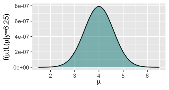
FIGURE 7.3: The unnormalized \(N(4,0.6^2)\) posterior pdf.

Further, Step 1 of the Metropolis-Hastings algorithm relies on the fact that, even when we don’t know and thus can’t sample from the posterior model, we can propose Markov chain tour stops by sampling from a different and more convenient model. As one of many options here, we’ll utilize a Uniform proposal model with half-width \(w\). Specifically, let \(\mu^{(i)} = \mu\) denote the current tour location. Conditioned on this current location, we propose the next location by taking a random draw \(\mu'\) from the Uniform model which is centered at the current location \(\mu\) and ranges from \(\mu - w\) to \(\mu + w\):

\[\mu' | \mu \; \sim \; \text{Unif}(\mu - w, \mu + w)\]

with pdf

\[q(\mu'|\mu) = \frac{1}{2w} \;\; \text{ for } \;\; \mu' \in [\mu - w, \mu + w] .\]

The Uniform pdf plotted in Figure 7.4 illustrates that, using this method, proposals \(\mu'\) are equally likely to be any value between \(\mu - w\) and \(\mu + w\).

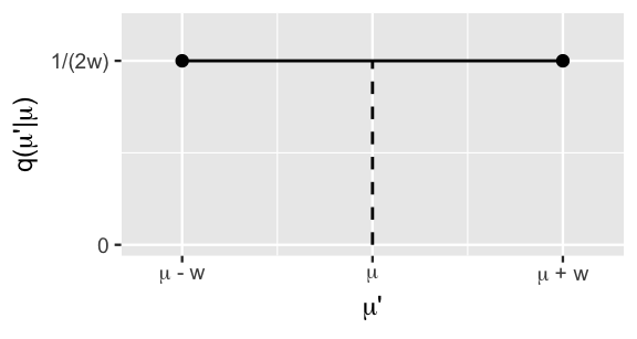
FIGURE 7.4: The Uniform proposal model.

Figure 7.5 illustrates this idea in a specific scenario. Suppose we’re utilizing a Uniform half-width of \(w = 1\) and that the Markov chain tour is at location \(\mu = 3\). Conditioned on this current location, we’ll then propose the next location by taking a random draw from a \(\text{Unif}(3-w, 3+w) = \text{Unif}(2,4)\) model. Thus, the chosen half-width \(w = 1\) plays an important role here, defining the neighborhood of potential proposals. Specifically, the proposed next stop is equally likely to be anywhere within the restricted neighborhood stretching from 2 to 4, around the chain’s current location of 3.

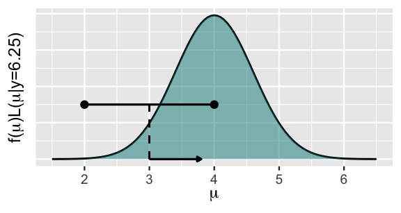
FIGURE 7.5: A visual representation of Step 1 in the Metropolis-Hastings algorithm for the N\((4,0.6^2)\) posterior. A Unif(2,4) proposal model centered at the current chain location of 3 (black curve) is drawn against the unnormalized posterior pdf.

The whole idea behind Step 1 might seem goofy. How can proposals drawn from a Uniform model produce a decent approximation of the Normal posterior model?!? Well, they’re only proposals. As with any other proposal in life, they can thankfully be rejected or accepted. Mainly, if a proposed location \(\mu'\) is “bad,” we can reject it. When we do, the chain sticks around at its current location \(\mu\) for at least another iteration.

Step 2 of the Metropolis-Hastings algorithm provides a formal process for deciding whether to accept or reject a proposal. Let’s first check in with our intuition about how this process should work. Revisiting Figure 7.5, suppose that our random Unif\((2, 4)\) draw proposes that the chain move from its current location of 3 to 3.8. Does this proposal seem desirable to you? Well, sure. Notice that the (unnormalized) posterior plausibility of 3.8 is greater than that of 3. Thus, we want our Markov chain tour to spend more time exploring values of \(\mu\) around 3.8 than around 3. Accepting the proposal gives us the chance to do so. In contrast, if our random Unif\((2, 4)\) draw proposed that the chain move from 3 to 2.1, a location with very low posterior plausibility, we might be more hesitant. Consider three possible rules for automating Step 2 in the following quiz.⁴¹

Suppose we start our Metropolis-Hastings Markov chain tour at location \(\mu^{(1)} = 3\) and utilize a Uniform proposal model in Step 1 of the algorithm. Consider three possible rules to follow in Step 2, deciding whether or not to accept a proposal:

• Rule 1: Never accept the proposed location.
• Rule 2: Always accept the proposed location.
• Rule 3: Only accept the proposed location if its (unnormalized) posterior plausibility is greater than that of the current location.

Each rule was used to generate one of the Markov chain tours in Figure 7.6. Match each rule to the correct tour.

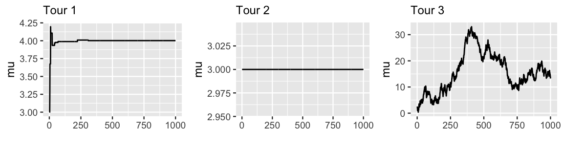
FIGURE 7.6: Trace plots corresponding to three different strategies for step 2 of the Metropolis-Hastings algorithm.

The quiz above presented you with three poor options for determining whether to accept or reject proposed tour stops in Step 2 of the Metropolis-Hastings algorithm. Rule 1 presents one extreme: never accept a proposal. This is a terrible idea. It results in the Markov chain remaining at the same location at every iteration (Tour 2), which would certainly produce a silly posterior approximation. Rule 2 presents the opposite extreme: always accept a proposal. This results in a Markov chain which is not at all discerning in where it travels (Tour 3), completely ignoring the information we have from the unnormalized posterior model regarding the plausibility of a proposal. For example, Tour 3 spends the majority of its time exploring posterior values \(\mu\) above 6, which we know from Figure 7.3 to be implausible.

Rule 3 might seem like a reasonable balance between the two extremes: it neither always rejects nor always accepts proposals. However, it’s still problematic. Since this rule only accepts a proposed stop if its posterior plausibility is greater than that at the current location, it ends up producing a Markov chain similar to that of Tour 1 above. Though this chain floats toward values near \(\mu = 4\), where the (unnormalized) posterior pdf is greatest, it then gets stuck there forever.

Putting all of this together, we’re closer to understanding how to make the Metropolis-Hastings algorithm work. Upon proposing a next tour stop (Step 1), the process for rejecting or accepting this proposal (Step 2) must embrace the idea that the chain should spend more time exploring areas of high posterior plausibility but shouldn’t get stuck there forever:

• Step 1: Propose a location, \(\mu'\), for the next tour stop by taking a draw from a proposal model.
• Step 2: Decide whether to go to the proposed location (\(\mu^{(i+1)} = \mu'\)) or to stay at the current location for another iteration (\(\mu^{(i+1)} = \mu\)) as follows.
  • If the (unnormalized) posterior plausibility of the proposed location \(\mu'\) is greater than that of the current location \(\mu\), \(f(\mu')L(\mu'|y) > f(\mu)L(\mu|y)\), definitely go there.
  • Otherwise, maybe go there.

There are more details to fill in here (e.g., what does it mean to “maybe” accept a proposal?!). We’ll do that next.

7.2 The Metropolis-Hastings algorithm

The Metropolis-Hastings algorithm for constructing a Markov chain tour \(\left\lbrace \mu^{(1)}, \mu^{(2)}, ..., \mu^{(N)}\right\rbrace\) is formalized here. We’ll break down the details below, exploring how to implement this algorithm in the context of our Normal-Normal Bayesian model.

Metropolis-Hastings algorithm

Conditioned on data \(y\), let parameter \(\mu\) have posterior pdf \(f(\mu | y) \propto f(\mu) L(\mu |y)\). A Metropolis-Hastings Markov chain for \(f(\mu|y)\), \(\left\lbrace \mu^{(1)}, \mu^{(2)}, ..., \mu^{(N)}\right\rbrace\), evolves as follows. Let \(\mu^{(i)} = \mu\) be the chain’s location at iteration \(i \in \{1,2,...,N-1\}\) and identify the next location \(\mu^{(i+1)}\) through a two-step process:

• Step 1: Propose a new location.
  Conditioned on the current location \(\mu\), draw a location \(\mu'\) from a proposal model with pdf \(q(\mu'|\mu)\).
  
• Step 2: Decide whether or not to go there.

  • Calculate the acceptance probability, i.e., the probability of accepting the proposal \(\mu'\):
    \[\begin{equation} \alpha = \min\left\lbrace 1, \; \frac{f(\mu')L(\mu'|y)}{f(\mu)L(\mu|y)} \frac{q(\mu|\mu')}{q(\mu'|\mu)} \right\rbrace. \tag{7.3} \end{equation}\]

  • Figuratively, flip a weighted coin. If it’s Heads, with probability \(\alpha\), go to the proposed location \(\mu'\). If it’s Tails, with probability \(1 - \alpha\), stay at \(\mu\):

    \[\mu^{(i+1)} = \begin{cases} \mu' & \text{ with probability } \alpha \\ \mu & \text{ with probability } 1- \alpha. \\ \end{cases}\]

Though the notation and details are new, the algorithm above matches the concepts we developed in the previous section. First, recall that for our Normal-Normal simulation, we utilized a \(\mu'|\mu \; \sim \text{Unif}(\mu - w, \mu + w)\) proposal model in Step 1. In fact, this is a bit lazy. Though our Normal-Normal posterior model is defined for \(\mu \in (-\infty, \infty)\), the Uniform proposal model lives on a truncated neighborhood around the current chain location. However, utilizing a Uniform proposal model simplifies the Metropolis-Hastings algorithm by the fact that it’s symmetric. This symmetry exhibits itself in the plot of the Uniform pdf (Figure 7.4), as well as numerically – the conditional pdf of \(\mu'\) given \(\mu\) is equivalent to that of \(\mu\) given \(\mu'\):

\[q(\mu'|\mu) = q(\mu|\mu') = \begin{cases} \frac{1}{2w} & \text{ when $\mu$ and $\mu'$ are within $w$ units of each other} \\ 0 & \text{ otherwise} \\ \end{cases} .\]

This symmetry means that the chance of proposing a chain move from \(\mu\) to \(\mu'\) is the same as proposing a move from \(\mu'\) to \(\mu\). For example, the Uniform model with a half-width of 1 is equally likely to propose a move from \(\mu = 3\) to \(\mu' = 3.8\) as a move from \(\mu = 3.8\) to \(\mu' = 3\). We refer to this special case of the Metropolis-Hastings algorithm as simply the Metropolis algorithm.

Metropolis algorithm

The Metropolis algorithm is a special case of the Metropolis-Hastings in which the proposal model is symmetric. That is, the chance of proposing a move to \(\mu'\) from \(\mu\) is equal to that of proposing a move to \(\mu\) from \(\mu'\): \(q(\mu'|\mu) = q(\mu|\mu')\). Thus, the acceptance probability (7.3) simplifies to

\[\begin{equation} \alpha = \min\left\lbrace 1, \; \frac{f(\mu')L(\mu'|y)}{f(\mu)L(\mu|y)} \right\rbrace . \tag{7.4} \end{equation}\]

Inspecting (7.4) reveals the nuances of Step 2, determining whether to accept or reject the proposed location drawn in Step 1. First, notice that we can rewrite the acceptance probability \(\alpha\) by dividing both the numerator and denominator by \(f(y)\):

\[\begin{equation} \alpha = \min\left\lbrace 1, \; \frac{f(\mu')L(\mu'|y) / f(y)}{f(\mu)L(\mu|y) / f(y)} \right\rbrace = \min\left\lbrace 1, \; \frac{f(\mu'|y)}{f(\mu|y)} \right\rbrace . \tag{7.5} \end{equation}\]

This rewrite emphasizes that, though we can’t calculate the posterior pdfs of \(\mu'\) and \(\mu\), \(f(\mu'|y)\) and \(f(\mu|y)\), their ratio is equivalent to that of the unnormalized posterior pdfs (which we can calculate). Thus, the probability of accepting a move from a current location \(\mu\) to a proposed location \(\mu'\) comes down to a comparison of their posterior plausibility: \(f(\mu'|y)\) versus \(f(\mu|y)\). There are two possible scenarios here:

• Scenario 1: \(f(\mu'|y) \ge f(\mu|y)\)
  When the posterior plausibility of \(\mu'\) is at least as great as that of \(\mu\), \(\alpha = 1\). Thus, we’ll definitely move there.

• Scenario 2: \(f(\mu'|y) < f(\mu|y)\)
  If the posterior plausibility of \(\mu'\) is less than that of \(\mu\), then

  \[\alpha = \frac{f(\mu'|y)}{f(\mu|y)} < 1 .\]

  Thus, we might move there. Further, \(\alpha\) approaches 1 as \(f(\mu'|y)\) nears \(f(\mu|y)\). That is, the probability of accepting the proposal increases with the plausibility of \(\mu'\) relative to \(\mu\).

Scenario 1 is straightforward. We’ll always jump at the chance to move our tour to a more plausible posterior region. To wrap our minds around Scenario 2, a little R simulation is helpful. For example, suppose our Markov tour is currently at location “3”:

current <- 3

Further, suppose we’re utilizing a Uniform proposal model with half-width \(w = 1\). Then to determine the next tour stop, we first propose a location by taking a random draw from the Unif(current - 1, current + 1) model (Step 1):

set.seed(8)
proposal <- runif(1, min = current - 1, max = current + 1)
proposal
[1] 2.933

Revisiting Figure 7.3, we observe that the (unnormalized) posterior plausibility of the proposed tour location (2.93) is slightly less than that of the current location (3). We can calculate the unnormalized posterior plausibility of these two \(\mu\) locations, \(f(\mu)L(\mu|y=6.25)\), using dnorm() to evaluate both pieces of the product:

• dnorm(..., 0, 1) calculates the N\((0,1^2)\) prior pdf \(f(\mu)\) at a given \(\mu\) value;
• dnorm(6.25, ..., 0.75) calculates the Normal likelihood function \(L(\mu|y=6.25)\) with \(Y = 6.25\) and standard deviation 0.75 at an unknown mean \(\mu\).

proposal_plaus <- dnorm(proposal, 0, 1) * dnorm(6.25, proposal, 0.75)
proposal_plaus
[1] 1.625e-07
current_plaus  <- dnorm(current, 0, 1) * dnorm(6.25, current, 0.75)
current_plaus
[1] 1.972e-07

It follows that, though not certain, the probability \(\alpha\) of accepting and subsequently moving to the proposed location is relatively high:

alpha <- min(1, proposal_plaus / current_plaus)
alpha
[1] 0.824

To make the final determination, we set up a weighted coin which accepts the proposal with probability \(\alpha\) (0.824) and rejects the proposal with probability \(1 - \alpha\) (0.176). In a random flip of this coin using the sample() function, we accept the proposal, meaning that the next_stop on the tour is 2.933:

next_stop <- sample(c(proposal, current),
                    size = 1, prob = c(alpha, 1-alpha))
next_stop
[1] 2.933

This is merely one of countless possible outcomes for a single iteration of the Metropolis-Hastings algorithm for our Normal posterior. To streamline this process, we’ll write our own R function, one_mh_iteration(), which implements a single Metropolis-Hastings iteration starting from any given current tour stop and utilizing a Uniform proposal model with any given half-width w. If you are new to writing functions, we encourage you to focus on the structure over the details of this code. Some things to pick up on:

• We first specify that one_mh_iteration is a function() of two arguments: the Uniform half-width w and the current chain value.
• We open and close the definition of the function with { }.
• Inside the function, we carry out the same steps as above and return() 3 pieces of information: the proposal, acceptance probability alpha, and next_stop.

one_mh_iteration <- function(w, current){
 # STEP 1: Propose the next chain location
 proposal <- runif(1, min = current - w, max = current + w)
  
 # STEP 2: Decide whether or not to go there
 proposal_plaus <- dnorm(proposal, 0, 1) * dnorm(6.25, proposal, 0.75)
 current_plaus  <- dnorm(current, 0, 1) * dnorm(6.25, current, 0.75)
 alpha <- min(1, proposal_plaus / current_plaus)
 next_stop <- sample(c(proposal, current), 
                     size = 1, prob = c(alpha, 1-alpha))
  
 # Return the results
 return(data.frame(proposal, alpha, next_stop))
}

Let’s try it out. Running one_mh_iteration() from our current tour stop of 3 under a seed of 8 reproduces the results from above:

set.seed(8)
one_mh_iteration(w = 1, current = 3)
  proposal alpha next_stop
1    2.933 0.824     2.933

If we use a seed of 83, the proposed next tour stop is 2.018, which has a low corresponding acceptance probability of 0.017:

set.seed(83)
one_mh_iteration(w = 1, current = 3)
  proposal   alpha next_stop
1    2.018 0.01709         3

This makes sense. We see from Figure 7.3 that the posterior plausibility of 2.018 is much lower than that of our current location of 3. Though we do want to explore such extreme values, we don’t want to do so often. In fact, we see that upon the flip of our coin, the proposal was rejected and the tour again visits location 3 on its next_stop. As a final example, we can confirm that when the posterior plausibility of the proposed next stop (here 3.978) is greater than that of our current location, the acceptance probability is 1 and the proposal is automatically accepted:

set.seed(7)
one_mh_iteration(w = 1, current = 3)
  proposal alpha next_stop
1    3.978     1     3.978

7.3 Implementing the Metropolis-Hastings

We’ve spent much energy understanding how to implement one iteration of the Metropolis-Hastings algorithm. That was the hard part! To construct an entire Metropolis-Hastings tour of our N\((4, 0.6^2)\) posterior, we now just have to repeat this process over and over and over. And by “we,” we mean the computer. To this end, the mh_tour() function below constructs a Metropolis-Hastings tour of any given length N utilizing a Uniform proposal model with any given half-width w:

mh_tour <- function(N, w){
  # 1. Start the chain at location 3
  current <- 3

  # 2. Initialize the simulation
  mu <- rep(0, N)

  # 3. Simulate N Markov chain stops
  for(i in 1:N){    
    # Simulate one iteration
    sim <- one_mh_iteration(w = w, current = current)
    
    # Record next location
    mu[i] <- sim$next_stop
    
    # Reset the current location
    current <- sim$next_stop
  }
  
  # 4. Return the chain locations
  return(data.frame(iteration = c(1:N), mu))
}

Again, this code is a big leap if you’re new to for loops and functions. Let’s focus on the general structure indicated by the # comment blocks. In one call to this function:

1. Start the tour at location 3, a somewhat arbitrary choice based on our prior understanding of \(\mu\).
2. Initialize the tour simulation by setting up an “empty” vector in which we’ll eventually store the N tour stops (mu).
3. Utilizing a for loop, at each tour stop \(i\) from 1 to N, run one_mh_iteration() and store the resulting next_stop in the ith element of the mu vector. Before closing the for loop, update the current tour stop to serve as a starting point for the next iteration.
4. Return a data frame with the iteration numbers and corresponding tour stops mu.

To see this function in action, use mh_tour() to simulate a Markov chain tour of length N = 5000 utilizing a Uniform proposal model with half-width \(w = 1\):

set.seed(84735)
mh_simulation_1 <- mh_tour(N = 5000, w = 1)

A trace plot and histogram of the tour results are shown below. Notably, this tour produces a remarkably accurate approximation of the N\((4, 0.6^2)\) posterior. You might need to step out of the weeds we’ve waded into in order to reflect upon the mathemagic here. Through a rigorous and formal process, we utilized dependent draws from a Uniform model to approximate a Normal model. And it worked!

ggplot(mh_simulation_1, aes(x = iteration, y = mu)) + 
  geom_line()

ggplot(mh_simulation_1, aes(x = mu)) + 
  geom_histogram(aes(y = ..density..), color = "white", bins = 20) + 
  stat_function(fun = dnorm, args = list(4,0.6), color = "blue")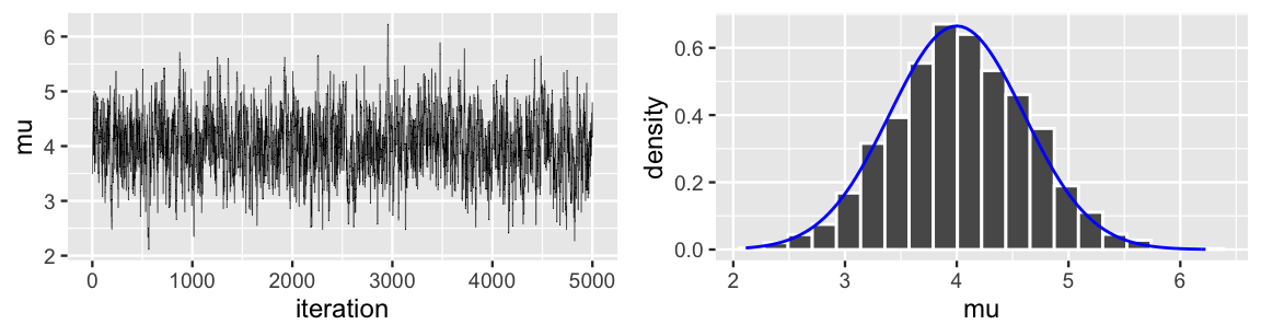

FIGURE 7.7: A trace plot (left) and histogram (right) of 5000 Metropolis chain values of \(\mu\). The target posterior pdf is superimposed in blue.

7.4 Tuning the Metropolis-Hastings algorithm

Let’s wade into one final weed patch. In implementing the Metropolis-Hastings algorithm above, we utilized a Uniform proposal model \(\mu' | \mu \; \sim \; \text{Unif}(\mu - w, \mu + w)\) with half-width \(w = 1\). Our selection of \(w = 1\) defined the neighborhood or range of potential proposals (Figure 7.5). Naturally, the choice of \(w\) impacts the performance of our Markov chain tour. Check your intuition about \(w\) with this quiz.

Figure 7.8 presents trace plots and histograms of three separate Metropolis-Hastings tours of the N\((4,0.6^2)\) posterior. Each tour utilizes a Uniform proposal model, but with different half-widths: \(w = 0.01\), \(w = 1\), or \(w = 100\). Match each tour to the \(w\) with which it was generated.

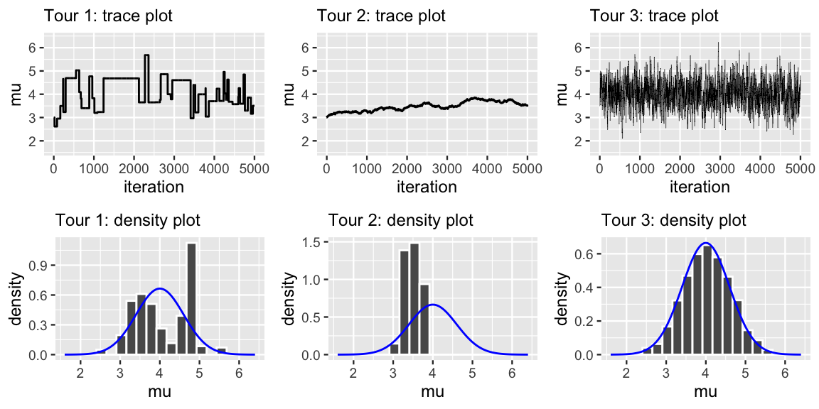
FIGURE 7.8: Trace plots (top row) and histograms (bottom row) for three different Metropolis-Hastings tours, where each tour utilizes a different proposal model. The shared target posterior pdf is superimposed in blue.

The answers are below.⁴² The main punchline is that the Metropolis-Hastings algorithm can work – we’ve seen as much – but we have to tune it. In our example, this means that we have to pick an appropriate half-width \(w\) for the Uniform proposal model. The tours in the quiz above illustrate the Goldilocks challenge this presents: we don’t want \(w\) to be too small or too large, but just right.⁴³ Tour 2 illustrates what can go wrong when \(w\) is too small (here \(w = 0.01\)). You can reproduce these results with the following code:

set.seed(84735)
mh_simulation_2 <- mh_tour(N = 5000, w = 0.01)
ggplot(mh_simulation_2, aes(x = iteration, y = mu)) + 
  geom_line() + 
  lims(y = c(1.6, 6.4))

In this case, the Uniform proposal model places a tight neighborhood around the tour’s current location – the chain can only move within 0.01 units at a time. Proposals will therefore tend to be very close to the current location, and thus have similar posterior plausibility and a high probability of being accepted. Specifically, when a proposal \(\mu' \approx \mu\), it’s typically the case that \(f(\mu')L(\mu'|y) \approx f(\mu)L(\mu|y)\) hence

\[\alpha = \min\left\lbrace 1, \; \frac{f(\mu')L(\mu'|y)}{f(\mu)L(\mu|y)} \right\rbrace \approx \min\left\lbrace 1, \; 1 \right\rbrace \; = 1 .\]

The result is a Markov chain that’s almost always moving, but takes such excruciatingly small steps that it will take an excruciatingly long time to explore the entire posterior plausible region of \(\mu\) values. Tour 1 illustrates the other extreme in which \(w\) is too large (here \(w = 100\)):

set.seed(7)
mh_simulation_3 <- mh_tour(N = 5000, w = 100)
ggplot(mh_simulation_3, aes(x = iteration, y = mu)) + 
  geom_line() + 
  lims(y = c(1.6,6.4))

By utilizing a Uniform proposal model with such a large neighborhood around the tour’s current location, proposals can be far flung – far outside the region of posterior plausible \(\mu\). In this case, proposals will often be rejected, resulting in a tour which gets stuck at the same location for multiple iterations in a row (as evidenced by the flat parts of the trace plot). Tour 3 presents a happy medium. This is our original tour (mh_simulation_1) which utilized \(w = 1\), a neighborhood size which is neither too small nor too big but just right. The corresponding tour efficiently explores the posterior plausible region of \(\mu\), not getting stuck in one place or region for too long.

7.5 A Beta-Binomial example

For extra practice, let’s implement the Metropolis-Hastings algorithm for a Beta-Binomial model in which we observe \(Y=1\) success in 2 trials:⁴⁴

\[\begin{split} Y|\pi & \sim \text{Bin}(2, \pi) \\ \pi & \sim \text{Beta}(2, 3) \\ \end{split} \;\; \Rightarrow \;\; \pi | (Y = 1) \sim \text{Beta}(3, 4) .\]

Again, pretend we were only able to define the posterior pdf up to some missing normalizing constant,

\[f(\pi | y = 1) \propto f(\pi) L(\pi | y = 1),\]

where \(f(\pi)\) is the Beta(2,3) prior pdf and \(L(\pi | y=1)\) is the \(\text{Bin}(2,\pi)\) likelihood function. Our goal then is to construct a Metropolis-Hastings tour of the posterior, \(\left\lbrace \pi^{(1)}, \pi^{(2)}, \ldots, \pi^{(N)}\right\rbrace\), utilizing a two-step iterative process: (1) at the current tour stop \(\pi\), take a random draw \(\pi'\) from a proposal model; and then (2) decide whether or not to move there. In step 1, the proposed tour stops would ideally be restricted to be between 0 and 1, just like \(\pi\) itself. Since the Uniform proposal model we used above might propose values outside this range, we’ll instead tune and utilize a \(\text{Beta}(a,b)\) proposal model. Further, we’ll utilize the same \(\text{Beta}(a,b)\) proposal model at each step in the chain. As such, our proposal strategy does not depend on the current tour stop (though whether or not we accept a proposal still will). This special case of the Metropolis-Hastings is referred to as the independence sampling algorithm.

Independence sampling algorithm

The independence sampling algorithm is a special case of the Metropolis-Hastings in which the same proposal model is utilized at each iteration, independent of the chain’s current location. That is, from a current location \(\pi\), a proposal \(\pi'\) is drawn from a proposal model with pdf \(q(\pi')\) (as opposed to \(q(\pi'|\pi)\)). Thus, the acceptance probability (7.3) simplifies to

\[\begin{equation} \alpha = \min\left\lbrace 1, \; \frac{f(\pi')L(\pi'|y)}{f(\pi)L(\pi|y)}\frac{q(\pi)}{q(\pi')} \right\rbrace . \tag{7.6} \end{equation}\]

We can rewrite \(\alpha\) for the independence sampler to emphasize its dependence on the relative posterior plausibility of proposal \(\pi'\) versus current location \(\pi\):

\[\begin{equation} \alpha = \min\left\lbrace 1, \; \frac{f(\pi')L(\pi'|y)/f(y)}{f(\pi)L(\pi|y)/f(y)}\frac{q(\pi)}{q(\pi')} \right\rbrace = \min\left\lbrace 1, \; \frac{f(\pi'|y)}{f(\pi|y)}\frac{q(\pi)}{q(\pi')} \right\rbrace . \tag{7.7} \end{equation}\]

Like the acceptance probability for the Metropolis algorithm (7.5), (7.7) includes the posterior pdf ratio \(f(\pi'|y)/f(\pi|y)\). This ensures that the independence sampler weighs the relative posterior plausibility of \(\pi'\) versus \(\pi\) in making its moves. Yet unlike the Metropolis acceptance probability, \(q(\pi)\) and \(q(\pi')\) aren’t typically equal, and thus do not cancel out of the formula. Rather, the inclusion of their ratio serves as a corrective measure: the probability \(\alpha\) of accepting a proposal \(\pi'\) decreases as \(q(\pi')\) increases. Conceptually, we place a penalty on common proposal values, ensuring that our tour doesn’t float toward these values simply because we keep proposing them.

The one_iteration() function below implements a single iteration of this independence sampling algorithm, starting from any current value \(\pi\) and utilizing a \(\text{Beta}(a,b)\) proposal model for any given a and b. In the calculation of acceptance probability \(\alpha\) (alpha), notice that we utilize dbeta() to evaluate the prior and proposal pdfs as well as dbinom() to evaluate the Binomial likelihood function with data \(Y = 1\), \(n = 2\), and unknown probability \(\pi\):

one_iteration <- function(a, b, current){
 # STEP 1: Propose the next chain location
 proposal <- rbeta(1, a, b)
  
 # STEP 2: Decide whether or not to go there
 proposal_plaus <- dbeta(proposal, 2, 3) * dbinom(1, 2, proposal)
 proposal_q     <- dbeta(proposal, a, b)
 current_plaus  <- dbeta(current, 2, 3) * dbinom(1, 2, current)
 current_q      <- dbeta(current, a, b)
 alpha <- min(1, proposal_plaus / current_plaus * current_q / proposal_q)
 next_stop <- sample(c(proposal, current), 
                     size = 1, prob = c(alpha, 1-alpha))
  
 return(data.frame(proposal, alpha, next_stop))
}

Subsequently, we write a betabin_tour() function which constructs an N-length Markov chain tour for any Beta(\(a, b\)) proposal model, utilizing one_iteration() to determine each stop:

betabin_tour <- function(N, a, b){
  # 1. Start the chain at location 0.5
  current <- 0.5

  # 2. Initialize the simulation
  pi <- rep(0, N)
  
  # 3. Simulate N Markov chain stops
  for(i in 1:N){    
    # Simulate one iteration
    sim <- one_iteration(a = a, b = b, current = current)
    
    # Record next location
    pi[i] <- sim$next_stop
    
    # Reset the current location
    current <- sim$next_stop
  }
  
  # 4. Return the chain locations
  return(data.frame(iteration = c(1:N), pi))
}

We encourage you to try different tunings of the \(\text{Beta}(a,b)\) proposal model. To keep it simple here, we run a 5,000 step tour of the Beta-Binomial posterior using a \(\text{Beta}(1,1)\), i.e., \(\text{Unif}(0,1)\), proposal model. As such, each proposal is equally likely to be anywhere between 0 and 1, no matter the chain’s current location. The results are summarized in Figure 7.9. You’re likely not surprised by now that this worked. The tour appears to be stable, random, and provides an excellent approximation of the Beta(3,4) posterior model (which in practice we wouldn’t have access to for comparison). That is, the Metropolis-Hastings algorithm allowed us to utilize draws from the Beta(1,1) proposal model to approximate our Beta(3,4) posterior. Cool.

set.seed(84735)
betabin_sim <- betabin_tour(N = 5000, a = 1, b = 1)

# Plot the results
ggplot(betabin_sim, aes(x = iteration, y = pi)) + 
  geom_line()
ggplot(betabin_sim, aes(x = pi)) + 
  geom_histogram(aes(y = ..density..), color = "white") + 
  stat_function(fun = dbeta, args = list(3, 4), color = "blue")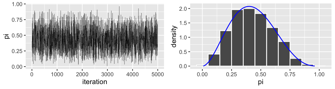

FIGURE 7.9: A trace plot (left) and histogram (right) for an independence sample of 5000 \(\pi\) values. The Beta(3,4) target posterior pdf is superimposed in blue.

7.6 Why the algorithm works

We’ve now seen how the Metropolis-Hastings algorithm works. But we haven’t yet discussed why it works. Though we’ll skip a formal proof, we’ll examine the underlying spirit. Throughout, consider constructing a Metropolis-Hastings tour of some generic posterior pdf \(f(\mu|y)\) utilizing a proposal pdf \(q(\mu'|\mu)\). For simplicity, let’s also assume \(\mu\) is a discrete variable. In general, the Metropolis-Hastings tour moves between different pairs of values, \(\mu\) and \(\mu'\). Specifically, the chain can move from \(\mu\) to \(\mu'\) with probability

\[P(\mu \to \mu') = P\left(\mu^{(i+1)}=\mu' \; | \; \mu^{(i)}=\mu \right)\]

or from \(\mu'\) to \(\mu\) with probability

\[P(\mu' \to \mu) = P\left(\mu^{(i+1)}=\mu \; | \; \mu^{(i)}=\mu' \right) .\]

In order for the Metropolis-Hastings algorithm to work (i.e., produce a good posterior approximation), its tour must preserve the relative posterior plausibility of any \(\mu'\) and \(\mu\) pair. That is, the relative probabilities of moving between these two values must satisfy

\[\frac{P(\mu \to \mu')}{P(\mu' \to \mu)} = \frac{f(\mu'|y)}{f(\mu|y)} .\]

This is indeed the case for any Metropolis-Hastings algorithm. And we can prove it. First, we need to calculate the movement probabilities \(P(\mu \to \mu')\) and \(P(\mu' \to \mu)\). Consider the former. For the tour to move from \(\mu\) to \(\mu'\), two things must happen: we need to propose \(\mu'\) and then accept the proposal. The associated probabilities of these two events are described by \(q(\mu'|\mu)\) and \(\alpha\) (7.3), respectively. It follows that the chain moves from \(\mu\) to \(\mu'\) with probability

\[P(\mu \to \mu') = q(\mu'|\mu) \cdot \min\left\lbrace 1, \; \frac{f(\mu'|y)}{f(\mu|y)} \frac{q(\mu|\mu')}{q(\mu'|\mu)} \right\rbrace .\]

Similarly, the chain moves from \(\mu'\) to \(\mu\) with probability

\[P(\mu' \to \mu) = q(\mu|\mu') \cdot \min\left\lbrace 1, \; \frac{f(\mu|y)}{f(\mu'|y)}\frac{q(\mu'|\mu)}{q(\mu|\mu')} \right\rbrace .\]

To simplify the ratio of movement probabilities \(P(\mu \to \mu') / P(\mu' \to \mu)\), consider the two potential scenarios:

1. Scenario 1: \(f(\mu'|y) \ge f(\mu|y)\)
   When \(\mu'\) is at least as plausible as \(\mu\), \(P(\mu \to \mu')\) simplifies to \(q(\mu'|\mu)\) and
   \[\frac{P(\mu \to \mu')}{P(\mu' \to \mu)} = \frac{q(\mu'|\mu)}{q(\mu|\mu') \frac{f(\mu|y)}{f(\mu'|y)}\frac{q(\mu'|\mu)}{q(\mu|\mu')} } = \frac{f(\mu'|y)}{f(\mu|y)} .\]

2. Scenario 2: \(f(\mu'|y) < f(\mu|y)\)
   When \(\mu'\) is less plausible than \(\mu\), \(P(\mu' \to \mu)\) simplifies to \(q(\mu|\mu')\) and

   \[\frac{P(\mu \to \mu')}{P(\mu' \to \mu)} = \frac{q(\mu'|\mu) \frac{f(\mu'|y)}{f(\mu|y)}\frac{q(\mu|\mu')}{q(\mu'|\mu)}}{q(\mu|\mu')} = \frac{f(\mu'|y)}{f(\mu|y)} .\]

Thus, no matter the scenario, the Metropolis-Hastings algorithm preserves the relative likelihood of any pair of values \(\mu\) and \(\mu'\)!

7.7 Variations on the theme

We’ve merely considered one MCMC algorithm here, the Metropolis-Hastings. Though powerful, this algorithm has its limits. In Chapter 7, we used the Metropolis-Hastings to simulate Normal-Normal and Beta-Binomial posteriors with single parameters \(\mu\) and \(\pi\), respectively. In future chapters, our Bayesian models will grow to include lots of parameters. Tuning a Metropolis-Hastings algorithm to adequately explore each of these parameters gets unwieldy. Yet even when it reaches its own limits of utility, the Metropolis-Hastings serves as the foundation for a more flexible set of MCMC tools, including the adaptive Metropolis-Hastings, Gibbs, and Hamiltonian Monte Carlo (HMC) algorithms. Among these, HMC is the algorithm utilized by the rstan and rstanarm packages.

As we noted at the top of Chapter 7, studying these alternative algorithms would require a book itself. From here on out, we’ll rely on rstan with a fresh confidence in what’s going on under the hood. If you’re curious to learn a little more, McElreath (2019) provides an excellent video introduction to the HMC algorithm and how it compares to the Metropolis-Hastings. For a deeper dive, Brooks et al. (2011) provides a comprehensive overview of the broader MCMC landscape.

7.8 Chapter summary

In Chapter 7, you built a strong conceptual understanding of the foundational Metropolis-Hastings MCMC algorithm. You also implemented this algorithm to study the familiar Normal-Normal and Beta-Binomial models. Whether in these relatively simple one-parameter model settings, or in more complicated model settings, the Metropolis-Hastings algorithm produces an approximate sample from the posterior by iterating between two steps:

1. Propose a new chain location by drawing from a proposal pdf which is, perhaps, dependent upon the current location.
2. Determine whether to accept the proposal. Simply put, whether or not we accept a proposal depends on how favorable its posterior plausibility is relative to the posterior plausibility of the current location.

7.9 Exercises

Chapter 7 continued to shift focus towards more computational methods. Change can be uncomfortable, but it also spurs growth. As you work through these exercises, know that if you are struggling a bit, that just means you are engaging with some new concepts and you are putting in the work to grow as a Bayesian. Our advice: verbalize what you do and don’t understand. Don’t rush yourself. Take a break and come back to exercises that you feel stuck on. Work with a buddy. Ask for help, and help others when you can.

7.9.1 Conceptual exercises

Exercise 7.1 (Getting to know Monte Carlo)

1. What are the steps to the Monte Carlo Algorithm?
2. Name one pro and one con for the Monte Carlo Algorithm.

Exercise 7.2 (Getting to know Metropolis-Hastings)

1. What are the steps to the Metropolis-Hastings Algorithm?
2. What’s the difference between the Monte Carlo and Metropolis-Hastings algorithms?
3. What’s the difference between the Metropolis and Metropolis-Hastings algorithms?

Exercise 7.3 (Metropolis vs Metropolis-Hastings) Select all of the correct endings to this sentence: The difference between the Metropolis and Metropolis-Hastings algorithms is that…

1. Metropolis accepts all proposals, whereas Metropolis-Hastings accepts only some proposals.
2. Metropolis uses a symmetric proposal model, whereas a Metropolis-Hastings proposal model is not necessarily symmetric.
3. The acceptance probability is simpler to calculate for the Metropolis than for the Metropolis-Hastings.

Exercise 7.4 (Tuning the Metropolis-Hastings) In this exercise you will consider how to tune a Uniform proposal model with half-width \(w\) for a Metropolis-Hastings algorithm.

1. Draw a trace plot for a tour where the Uniform proposal model uses a very small \(w\).
2. Why is it problematic if \(w\) is too small, and hence defines the neighborhood around the current chain value too narrowly?
3. Draw a trace plot for a tour where the Uniform proposal model uses a very large \(w\).
4. Why is it problematic if \(w\) is too large, and hence defines the neighborhood too widely?
5. Draw a trace plot for a tour where the Uniform proposal model uses a \(w\) that is neither too small or too large.
6. Describe how you would go about finding an appropriate half-width \(w\) for a Uniform proposal model.

Exercise 7.5 (Independence sampling: True or False) Identify whether the below statements about independence sampling are True or False. If False, explain.

1. The proposal model depends on the current value of the chain.
2. The proposal model is the same every time.
3. It is a special case of the Metropolis-Hastings algorithm.
4. It is a special case of Metropolis algorithm.

Exercise 7.6 (Proposing a new location) In each situation below, complete Step 1 of the Metropolis-Hastings Algorithm. That is, starting from the given current chain value \(\lambda^{(i)} = \lambda\) and with set.seed(84735), use the given proposal model to draw a \(\lambda'\) proposal value for the next chain value \(\lambda^{(i+1)}\).

1. \(\lambda = 4.6\), \(\lambda'|\lambda \sim N(\lambda, 2^2)\)
2. \(\lambda = 2.1\), \(\lambda'|\lambda \sim N(\lambda, 7^2)\)
3. \(\lambda = 8.9\), \(\lambda'|\lambda \sim \text{Unif}(\lambda-2, \lambda+2)\)
4. \(\lambda = 1.2\), \(\lambda'|\lambda \sim \text{Unif}(\lambda-0.5, \lambda+0.5)\)
5. \(\lambda = 7.7\), \(\lambda'|\lambda \sim \text{Unif}(\lambda-3, \lambda+3)\)

Exercise 7.7 (Calculate the acceptance probability: Part I) Suppose that a Markov chain is currently at \(\lambda^{(i)}=2\) and that the proposal for \(\lambda^{(i+1)}\) is \(\lambda'=2.1\). For each pair of unnormalized posterior pdf \(f(\lambda) L(\lambda |y)\) and proposal pdf \({q(\lambda'|\lambda)}\), calculate the acceptance probability \(\alpha\) used in Step 2 of the Metropolis-Hastings algorithm (7.3).

1. \(f(\lambda) L(\lambda |y)= \lambda^{-2}\), \({\lambda'|\lambda} \sim \text{N}(\lambda, 1^2)\) with pdf \(q(\lambda'|\lambda)\)
2. \(f(\lambda) L(\lambda |y)= e^{\lambda}\), \({\lambda'|\lambda} \sim \text{N}(\lambda, 0.2^2)\) with pdf \(q(\lambda'|\lambda)\)
3. \(f(\lambda) L(\lambda |y)= e^{-10\lambda}\), \({\lambda'|\lambda} \sim \text{Unif}(\lambda - 0.5, \lambda + 0.5)\) with pdf \(q(\lambda'|\lambda)\)
4. \(f(\lambda) L(\lambda |y)= e^{-\lambda^4}\), \({\lambda'|\lambda} \sim \text{Exp}(\lambda)\) with pdf \(q(\lambda'|\lambda)\)
5. For which of these scenarios is there a 100% acceptance probability? Explain why we’d certainly want to accept \(\lambda'\) in these scenarios.

Exercise 7.8 (Calculate the acceptance probability: Part II) Suppose that a Markov chain is currently at \(\lambda^{(i)}=1.8\) and that the proposal for \(\lambda^{(i+1)}\) is \(\lambda'=1.6\). For each pair of unnormalized posterior pdf \(f(\lambda) L(\lambda |y)\) and proposal pdf \({q(\lambda'|\lambda)}\), calculate the acceptance probability \(\alpha\) used in Step 2 of the Metropolis-Hastings algorithm (7.3).

1. \(f(\lambda) L(\lambda |y)= \lambda^{-1}\), \({\lambda'|\lambda} \sim \text{N}(\lambda, 2^2)\) with pdf \(q(\lambda'|\lambda)\)
2. \(f(\lambda) L(\lambda |y)= e^{3\lambda}\), \({\lambda'|\lambda} \sim \text{N}(\lambda, 0.5^2)\) with pdf \(q(\lambda'|\lambda)\)
3. \(f(\lambda) L(\lambda |y)= e^{-1.9\lambda}\), \({\lambda'|\lambda} \sim \text{Unif}(\lambda-0.3, \lambda+0.3)\) with pdf \(q(\lambda'|\lambda)\)
4. \(f(\lambda) L(\lambda |y)= e^{-\lambda^4}\), \({\lambda'|\lambda} \sim \text{Exp}(\lambda)\) with pdf \(q(\lambda'|\lambda)\)
5. For which of these scenarios is there a 100% acceptance probability? Explain why we’d certainly want to accept \(\lambda'\) in these scenarios.

7.9.2 Practice: Normal-Normal simulation

In the next set of exercises, return to the Bayesian model setting of (7.1),

\[\begin{split} Y|\mu & \sim \text{N}(\mu, 0.75^2) \\ \mu & \sim \text{N}(0, 1^2). \\ \end{split}\]

Assume we observe \(Y = 6.25\) and wish to construct a Metropolis-Hastings simulation of the corresponding posterior model for \(\lambda\).

Exercise 7.9 (One iteration with a Uniform proposal model) The function one_mh_iteration() from the text utilizes a Uniform proposal model, \(\mu'|\mu \sim \text{Unif}(\mu - w, \mu + w)\) with half-width \(w = 1\). Starting from a current value of \(\mu = 3\) and using set.seed(1), run the code below and comment on the returned proposal, alpha, and next_stop values.

1. one_mh_iteration(w = 0.01, current = 3)
2. one_mh_iteration(w = 0.5, current = 3)
3. one_mh_iteration(w = 1, current = 3)
4. one_mh_iteration(w = 3, current = 3)

Exercise 7.10 (An entire tour with a Uniform proposal model) Implement the Metropolis-Hastings function mh_tour() defined in Section 7.3 to construct tours of \(\mu\) under each of the following scenarios. Construct trace plots and histograms for each tour.

1. 50 iterations, \(w = 50\)
2. 50 iterations, \(w = 0.01\)
3. 1000 iterations, \(w = 50\)
4. 1000 iterations, \(w = 0.01\)
5. Contrast the trace plots in parts a and b. Explain why changing \(w\) has this effect.
6. Consider the results in parts c and d. Is the \(w\) value as important when the number of iterations is much larger? Explain.

Exercise 7.11 (Changing the proposal model) For this exercise, modify one_mh_iteration() to create a new function, one_mh_iteration_normal(), which utilizes a symmetric Normal proposal model, centered at the current chain value \(\mu\) with standard deviation \(s\):

\[\mu'|\mu \sim N(\mu, s^2).\]

Subsequently, starting from a current value of \(\mu = 3\) and set.seed(1), run this function under each setting below. Comment on the returned proposal, alpha, and next_stop values.

1. one_mh_iteration_normal(s = 0.01, current = 3)
2. one_mh_iteration_normal(s = 0.5, current = 3)
3. one_mh_iteration_normal(s = 1, current = 3)
4. one_mh_iteration_normal(s = 3, current = 3)

Exercise 7.12 (Metropolis-Hastings tour with Normal proposals) Upon completing the previous exercise, modify mh_tour() to create a new function, mh_tour_normal(), which constructs a chain of \(\mu\) values using a Normal proposal model with standard deviation \(s\). Subsequently, using set.seed(84735), run this function under each setting below and construct a trace plot of the chain.

1. 20 iterations, \(s = 0.01\)
2. 20 iterations, \(s = 10\)
3. 1000 iterations, \(s = 0.01\)
4. 1000 iterations, \(s = 10\)
5. Contrast the trace plots in a and b. Explain in simple terms why changing the standard deviation of the Normal proposal model causes these differences.
6. Reflecting on the above results, tune your Metropolis-Hastings algorithm. That is, identify a reasonable value for standard deviation \(s\) and provide a trace plot as proof.

Exercise 7.13 (Change the Normal prior) The one_mh_iteration(w, current) function from the text is tailored to the Normal-Normal model (7.1) with a \(N(0,1^2)\) prior for \(\mu\). For this exercise, create a new function new_mh_iteration(w, current, m, s) which can utilize any \(N(m,s^2)\) prior. Subsequently, starting from a current value of \(\mu = 3\) and using set.seed(84735), run this function under each setting below. Comment on the resulting proposal, alpha, and next_stop values.

1. new_mh_iteration(w = 1, current = 3, m = 0, s = 10)
2. new_mh_iteration(w = 1, current = 3, m = 20, s = 1)
3. new_mh_iteration(w = 0.1, current = 3, m = 20, s = 1)
4. new_mh_iteration(w = 0.1, current = 3, m = -15, s = 10)

Exercise 7.14 (A Gamma-Poisson model) Consider a Gamma-Poisson model in which rate \(\lambda\) has a Gamma(1,0.1) prior and you observe one Poisson data point, \(Y = 4\). In this exercise, you will simulate the posterior model of \(\lambda\) using an independence sampler.

1. Which of the following would make the most reasonable proposal model to use in your independence sampler for \(\lambda\): Normal, Beta, or Exponential? Hint: Recall that \(\lambda > 0\).
2. Using the proposal model that you identified in part a, simulate a tour of 1000 \(\lambda\) values. Tune your algorithm until you are satisfied and produce a trace plot of your final results.
3. This is a situation where we can derive the exact posterior model of \(\lambda\). What is it?
4. Plot a histogram of your tour and overlay the exact model. How good is your Markov chain approximation?

7.9.3 Practice: Simulating more Bayesian models

In this section you will apply your new simulation skills to answer your own research question using your own data! In each case, identify a question for which data collection takes fewer than 5 minutes of effort. (That part is supposed to be fun, not overwhelming.)

Exercise 7.15 (Using your own data: Beta-Binomial Metropolis-Hastings)

1. Identify a question that could be answered with a Beta-Binomial model for \(\pi\), some probability or proportion of interest. Consider scenarios for which data collection would be easy, such as the proportion of emails that you reply to within 24 hours, the proportion of phone calls that you answer, etc.
2. Tune and describe a Beta prior model for \(\pi\).
3. Collect and record your data here.
4. Below you will simulate the posterior model of \(\pi\) using a Metropolis-Hastings algorithm. What is a reasonable proposal model to use in this algorithm? Explain.
5. Simulate a tour of 2000 \(\pi\) values. Tune your proposal model until you are satisfied and construct the resulting trace plot.
6. Plot a histogram of your tour, and comment on the posterior model approximation within the context of your question.

Exercise 7.16 (Using your own data: Normal-Normal MCMC)

1. Identify a question that could be answered with a Normal-Normal model for \(\mu\), some average of interest. Consider scenarios for which data collection would be easy, such as the average high temperature this time of year, your average hourly screen time, etc.
2. Tune and describe a Normal prior model for \(\mu\).
3. Collect and record your data here.
4. Below you will simulate the posterior model of \(\mu\) using a Metropolis-Hastings algorithm. What is a reasonable proposal model to use in this algorithm? Explain.
5. Simulate a tour of 2000 \(\mu\) values. Tune your proposal model until you are satisfied and construct the resulting trace plot.
6. Plot a histogram of your tour, and comment on the posterior model approximation within the context of your question.

Exercise 7.17 (Using your own data: Normal-Normal Independence Sampler) Repeat the previous exercise, this time using an independence sampler.

References

Brooks, Steve, Andrew Gelman, Galin Jones, and Xiao-Li Meng. 2011. Handbook of Markov Chain Monte Carlo. CRC Press.

McElreath, Richard. 2019. “Statistical Rethinking Winter 2019 Lecture 12.” Youtube; https://www.youtube.com/watch?v=hRJtKCIDTwc.

---

41. Answers: Rule 1 produces Tour 2, Rule 2 produces Tour 3, and Rule 3 produces Tour 1.↩︎

42. Answers: Tour 1 uses \(w = 100\), Tour 2 uses \(w = 0.01\), Tour 3 uses \(w = 1\).↩︎

43. This technical term was inspired by the “Goldilocks and the three bears” fairy tale in which, for some reason, a child (Goldilocks) taste tests three different bears’ porridge while trespassing in the bears’ house. The first bowl of porridge is too hot, the second is too cold, and the third is just right.↩︎

44. By Chapter 3, the Beta posterior has parameters 3 (\(\alpha + y = 2 + 1\)) and 4 (\(\beta + n - y = 3 + 2 - 1\)).↩︎