Chapter 9 Simple Normal Regression

Welcome to Unit 3!

Our work in Unit 1 (learning how to think like Bayesians and build simple Bayesian models) and Unit 2 (exploring how to simulate and analyze these models), sets us up to expand our Bayesian toolkit to more sophisticated models in Unit 3. Thus, far, our models have focused on the study of a single data variable \(Y\). For example, in Chapter 4 we studied \(Y\), whether or not films pass the Bechdel test. Yet once we have a grip on the variability in \(Y\), we often have follow-up questions: can the passing / failing of the Bechdel test be explained by a film’s budget, genre, release date, etc.?

In general, we often want to model the relationship between some response variable \(Y\) and predictors (\(X_1,X_2,...,X_p\)). This is the shared goal of the remaining chapters, which will survey a broad set of Bayesian modeling tools that we conventionally break down into two tasks:

• Regression tasks are those that analyze and predict quantitative response variables (e.g., \(Y\) = hippocampal volume).
• Classification tasks are those that analyze categorical response variables with the goal of predicting or classifying the response category (e.g., classify \(Y\), whether a news article is real or fake).

We’ll survey a few Bayesian regression techniques in Chapters 9 through 12: Normal, Poisson, and Negative Binomial regression. We’ll also survey two Bayesian classification techniques in Chapters 13 and 14: logistic regression and naive Bayesian classification. Though we can’t hope to introduce you to every regression and classification tool you’ll ever need, the five we’ve chosen here are generalizable to a broader set of applications. At the outset of this exploration, we encourage you to focus on the Bayesian modeling principles. By focusing on principles over a perceived set of rules (which don’t exist), you’ll empower yourself to extend and apply what you learn here beyond the scope of this book.

In Chapter 9 we’ll start with the foundational Normal regression model for a quantitative response variable \(Y\). Consider the following data story. Capital Bikeshare is a bike sharing service in the Washington, D.C. area. To best serve its registered members, the company must understand the demand for its service. To help them out, we can analyze the number of rides taken on a random sample of \(n\) days, (\(Y_1, Y_2, ..., Y_n\)). Since \(Y_i\) is a count variable, you might assume that ridership might be well modeled by a Poisson. However, past bike riding seasons have exhibited bell-shaped daily ridership with a variability in ridership that far exceeds the typical ridership, grossly violating the Poisson assumption of equal mean and variance (5.4). Thus, we’ll assume instead that, independently from day to day, the number of rides varies normally around some typical ridership, \(\mu\), with standard deviation \(\sigma\) (Figure 9.1): \(Y_i | \mu, \sigma \stackrel{ind}{\sim} N(\mu, \sigma^2) .\)

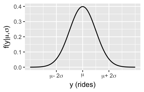
FIGURE 9.1: A Normal model of bike ridership.

Utilizing the Normal-Normal model from Chapter 5, we could conduct a posterior analysis of the typical ridership \(\mu\) in light of the observed data by (1) tuning a Normal prior model for \(\mu\); and (2) assuming the variability in ridership \(\sigma\) is known:

\[\begin{equation} \begin{split} Y_i | \mu & \stackrel{ind}{\sim} N(\mu, \sigma^2)\\ \mu & \sim N(\theta, \tau^2) .\\ \end{split} \tag{9.1} \end{equation}\]

Yet we can greatly extend the power of this model by tweaking its assumptions. First, you might have scratched your head at the assumption that we don’t know the typical ridership \(\mu\) but do know the variability in ridership from day to day, \(\sigma\). You’d be right. This assumption typically breaks down outside textbook examples. No problem. We can generalize the Normal-Normal model (9.1) to accommodate the reality that \(\sigma\) is a second unknown parameter by including a corresponding prior model:

\[\begin{equation} \begin{split} Y_i | \mu, \sigma & \stackrel{ind}{\sim} N(\mu, \sigma^2)\\ \mu & \sim N(\theta, \tau^2) \\ \sigma & \sim \text{ some prior model.} \\ \end{split} \tag{9.2} \end{equation}\]

We can do even better. Though this two-parameter Normal-Normal model is more flexible than the one-parameter model (9.1), it ignores a lot of potentially helpful information. After all, ridership is likely linked to factors or predictors such as the weather, day of the week, time of the year, etc. In Chapter 9 we’ll focus on incorporating just one predictor into our analysis – temperature – which we’ll label as \(X\). Specifically, our goal will be to model the relationship between ridership and temperature: Does ridership tend to increase on warmer days? If so, by how much? And how strong is this relationship? Figuring out how to conduct this analysis, i.e., how exactly to get information about the temperature predictor (\(X\)) into our model of ridership (\(Y\)) (9.2), is the driver behind Chapter 9.

Upon building a Bayesian simple linear regression model of response variable \(Y\) versus predictor \(X\), you will:

• interpret appropriate prior models for the regression parameters;
• simulate the posterior model of the regression parameters; and
• utilize simulation results to build a posterior understanding of the relationship between \(Y\) and \(X\) and to build posterior predictive models of \(Y\).

To get started, load the following packages, which we’ll utilize throughout the chapter:

# Load packages
library(bayesrules)
library(tidyverse)
library(rstan)
library(rstanarm)
library(bayesplot)
library(tidybayes)
library(janitor)
library(broom.mixed)

9.1 Building the regression model

In this section, we build up the framework of the Normal Bayesian regression model. These concepts will be solidified when applied to the bike data in Section 9.3.

9.1.1 Specifying the data model

Our analysis of the relationship between bike ridership (\(Y\)) and temperature (\(X\)) requires a sample of \(n\) data pairs,

\[\left\lbrace (Y_1,X_1), (Y_2,X_2),...,(Y_n,X_n) \right\rbrace\]

where \(Y_i\) is the number of rides and \(X_i\) is the high temperature (in degrees Fahrenheit) on day \(i\). We can check this assumption once we have some data, but our experience suggests there’s a positive linear relationship between ridership and temperature – the warmer it is, the more likely people are to hop on their bikes. For example, we might see data like that in the two scenarios in Figure 9.2 where each dot reflects the ridership and temperature on a unique day. Thus, instead of focusing on the global mean ridership across all days combined (\(\mu\)), we can refine our analysis to the local mean ridership on day \(i\), \(\mu_i\), specific to the temperature on that day. Assuming the relationship between ridership and temperature is linear, we can write \(\mu_i\) as

\[\mu_i = \beta_0 + \beta_1 X_i\]

where we can interpret the model coefficients \(\beta_0\) and \(\beta_1\) as follows:

• Intercept coefficient \(\beta_0\) technically indicates the typical ridership on days in which the temperature was 0 degrees Fahrenheit (\(X_i = 0\)). Since this frigid temperature is far outside the norm for D.C., we shouldn’t put stock into this interpretation. Rather, we can think of \(\beta_0\) as providing a baseline for where our model “lives” along the y-axis.
• Temperature coefficient \(\beta_1\) indicates the typical change in ridership for every one unit (degree) increase in temperature. In this particular model with only one quantitative predictor \(X\), this coefficient is equivalent to a slope.

For example, the model lines in Figure 9.2 both have intercept \(\beta_0 = -2000\) and slope \(\beta_1 = 100\). The intercept just tells us that if we extended the line all the way down to 0 degrees Fahrenheit, it would cross the y-axis at -2000. The slope is more meaningful, indicating that for every degree increase in temperature, we’d expect 100 more riders.

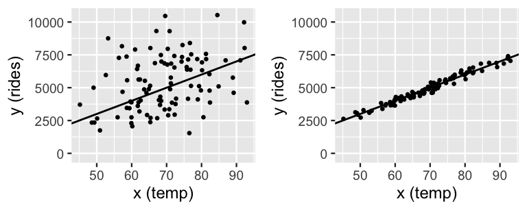
FIGURE 9.2: Two simulated scenarios for the relationship between ridership and temperature, utilizing \(\sigma = 2000\) (left) and \(\sigma = 200\) (right). In both cases, the model line is defined by \(\beta_0 + \beta_1 x = -2000 + 100 x\).

We can plunk this assumption of a linear relationship between \(Y_i\) and \(X_i\) right into our Bayesian model, by replacing the global mean \(\mu\) in the Normal data model, \(Y_i | \mu,\sigma \sim N(\mu, \sigma^2)\), with the temperature specific local mean \(\mu_i\):

\[\begin{equation} \begin{split} Y_i | \beta_0, \beta_1, \sigma & \stackrel{ind}{\sim} N\left(\mu_i, \sigma^2\right) \;\; \text{ with } \;\; \mu_i = \beta_0 + \beta_1X_i .\\ \end{split} \tag{9.3} \end{equation}\]

In this formulation of the data model, \(\sigma\) also takes on new meaning. It no longer measures the variability in ridership from the global mean \(\mu\) across all days, but the variability from the local mean on days with similar temperature, \(\mu_i = \beta_0 + \beta_1 X_i\). Pictures help. In Figure 9.2, the right plot reflects a scenario with a relatively small value of \(\sigma = 20\). The observed data here deviates very little from the mean model line – we can expect the observed ridership on a given day to differ by only 20 rides from the mean ridership on days of the same temperature. This tightness around the mean model line indicates that temperature is a strong predictor of ridership. The opposite is true in the left plot which exhibits a larger \(\sigma = 200\). There is quite a bit of variability in ridership among days of the same temperature, reflecting a weaker relationship between these variables. In summary, the formal assumptions encoded by data model (9.3) are included below.

Normal regression assumptions

The appropriateness of the Bayesian Normal regression model (9.3) depends upon the following assumptions.

• Structure of the data
  Accounting for predictor \(X\), the observed data \(Y_i\) on case \(i\) is independent of the observed data on any other case \(j\).
• Structure of the relationship
  The typical \(Y\) outcome can be written as a linear function of predictor \(X\), \(\mu = \beta_0 + \beta_1 X\).
• Structure of the variability
  At any value of predictor \(X\), the observed values of \(Y\) will vary normally around their average \(\mu\) with consistent standard deviation \(\sigma\).

9.1.2 Specifying the priors

Considered alone, the modified data model (9.3) is precisely the frequentist “simple” linear regression model that you might have studied outside this book⁴⁶ – “simple” here meaning that our model has only one predictor variable \(X\), not that you should find this model easy. To turn this into a Bayesian model, we must incorporate prior models for each of the unknown regression parameters. To practice distinguishing between model parameters and data variables, take the following quiz.⁴⁷

Identify the regression parameters upon which the data model (9.3) depends.

In the data model (9.3), there are two data variables (\(Y\) and \(X\)) and three unknown regression parameters that encode the relationship between these variables: \(\beta_0,\beta_1,\sigma\). We must specify prior models for each. There are countless approaches to this task. We won’t and can’t survey them all. Rather, throughout this book we’ll utilize the default framework of the prior models used by the rstanarm package. Working within this framework will allow us to survey a broad range of modeling tools in Units 3 and 4. Once you’re comfortable with the general modeling concepts therein and are ready to customize, you can take that leap. In doing so, we recommend Gabry and Goodrich (2020b), which provides an overview of all possible prior structures in rstanarm.

The first assumption we’ll make is that our prior models of \(\beta_0\), \(\beta_1\), and \(\sigma\) are independent. That is, we’ll assume that our prior understanding of where the model “lives” (\(\beta_0\)) has nothing to do with our prior understanding of the rate at which ridership increases with temperature (\(\beta_1\)). Similarly, we’ll assume that our prior understanding of \(\sigma\), and hence the strength of the relationship, is unrelated to both \(\beta_0\) and \(\beta_1\). Though in practice we might have some prior notion about the combination of these parameters, the assumption of independence greatly simplifies the model. It’s also consistent with the rstanarm framework.

In specifying the structure of the independent priors, we must consider (as usual) the values that these parameters might take. To this end, the intercept and slope regression parameters, \(\beta_0\) and \(\beta_1\), can technically take any values in the real line. That is, a model line can cross anywhere along the y-axis and the slope of a line can be any positive or negative value (or even 0). Thus, it’s reasonable to utilize Normal prior models for \(\beta_0\) and \(\beta_1\), which also live on the entire real line. Specifically,

\[\begin{equation} \begin{split} \beta_0 & \sim N\left(m_0, s_0^2 \right) \\ \beta_1 & \sim N\left(m_1, s_1^2 \right) \\ \end{split} \tag{9.4} \end{equation}\]

where we can tune the \(m_0\), \(s_0\), \(m_1\), \(s_1\) hyperparameters to match our prior understanding of \(\beta_0\) and \(\beta_1\). Similarly, since the standard deviation parameter \(\sigma\) must be positive, it’s reasonable to utilize an Exponential model which is also restricted to positive values:

\[\begin{equation} \begin{split} \sigma & \sim \text{Exp}(l) .\\ \end{split} \tag{9.5} \end{equation}\]

Thus, by (5.9), the prior mean and standard deviation of \(\sigma\) are:

\[E(\sigma) = \frac{1}{l} \;\; \text{ and } \;\; SD(\sigma) = \frac{1}{l}.\]

Though this Exponential prior is currently the default in rstanarm, popular alternatives include the half-Cauchy and inverted Gamma models.

9.1.3 Putting it all together

Combining the Normal data model (9.3) with our priors on the model parameters, (9.4) and (9.5), completes a common formulation of the Bayesian simple linear regression model:

\[\begin{equation} \begin{array}{lcrl} \text{data:} & \hspace{.05in} & Y_i | \beta_0, \beta_1, \sigma & \stackrel{ind}{\sim} N\left(\mu_i, \sigma^2\right) \;\; \text{ with } \;\; \mu_i = \beta_0 + \beta_1X_i \\ \text{priors:} & & \beta_0 & \sim N\left(m_0, s_0^2 \right) \\ & & \beta_1 & \sim N\left(m_1, s_1^2 \right) \\ & & \sigma & \sim \text{Exp}(l) .\\ \end{array} \tag{9.6} \end{equation}\]

Step back and reflect upon how we got here. We built a regression model of \(Y\), not all at once, but by starting with and building upon the simple Normal-Normal model one step at a time. In contrast, our human instinct often draws us into starting with the most complicated model we can think of. When this instinct strikes, resist it and remember this: complicated is not necessarily sophisticated. Complicated models are often wrong and difficult to apply.

Model building: One step at a time

In building any Bayesian model, it’s important to start with the basics and build up one step at a time. Let \(Y\) be a response variable and \(X\) be a predictor or set of predictors. Then we can build a model of \(Y\) by \(X\) through the following general principles:

• Take note of whether \(Y\) is discrete or continuous. Accordingly, identify an appropriate model structure of data \(Y\) (e.g., Normal, Poisson, Binomial).
• Rewrite the mean of \(Y\) as a function of predictors \(X\) (e.g., \(\mu = \beta_0 + \beta_1 X\)).
• Identify all unknown model parameters in your model (e.g., \(\beta_0, \beta_1, \sigma\)).
• Take note of the values that each of these parameters might take. Accordingly, identify appropriate prior models for these parameters.

9.2 Tuning prior models for regression parameters

Let’s now apply the Bayesian simple linear regression model (9.6) to our study of the relationship between Capital Bikeshare ridership (\(Y\)) and temperature (\(X\)). We’ll begin by tuning the prior models for intercept coefficient \(\beta_0\), temperature coefficient \(\beta_1\), and regression standard deviation \(\sigma\). Based on past bikeshare analyses, suppose we have the following prior understanding of this relationship:

1. On an average temperature day, say 65 or 70 degrees for D.C., there are typically around 5000 riders, though this average could be somewhere between 3000 and 7000.

2. For every one degree increase in temperature, ridership typically increases by 100 rides, though this average increase could be as low as 20 or as high as 180.

3. At any given temperature, daily ridership will tend to vary with a moderate standard deviation of 1250 rides.

Prior assumption 1 tells us something about the model baseline or intercept, \(\beta_0\). There’s a twist though. This prior information has been centered. Whereas \(\beta_0\) reflects the typical ridership on a 0-degree day (which doesn’t make sense in D.C.), the centered intercept, which we’ll denote \(\beta_{0c}\), reflects the typical ridership at the typical temperature \(X\). The distinction between \(\beta_0\) and \(\beta_{0c}\) is illustrated in Figure 9.3. Processing the prior information about the model baseline in this way is more intuitive. In fact, it’s this centered information that we’ll supply when using rstanarm to simulate our regression model. With this, we can capture prior assumption 1 with a Normal model for \(\beta_{0c}\) which is centered at 5000 rides with a standard deviation of 1000 rides, and thus largely falls between 3000 and 7000 rides: \(\beta_{0c} \sim N(5000, 1000^2)\). This prior is drawn in Figure 9.4.

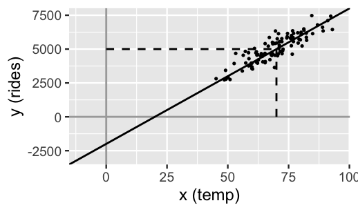
FIGURE 9.3: A simulated set of ridership data with intercept \(\beta_0 = -2000\) and centered intercept \(\beta_{0c} = 5000\) at an average temperature of 70 degrees.

Moving on, prior assumption 2 tells us about the rate of increase in ridership with temperature, and thus temperature coefficient \(\beta_1\). This prior understanding is well represented by a Normal model centered at 100 with a standard deviation of 40, and thus largely falls between 20 and 180: \(\beta_1 \sim N(100, 40^2)\). Finally, prior assumption 3 reflects our understanding of the regression standard deviation parameter \(\sigma\). Accordingly, we can tune the Exponential model to have a mean that matches the expected standard deviation of \(E(\sigma) = 1/l = 1250\) rides, and thus a rate of \(l = 1/1250 = 0.0008\): \(\sigma \sim \text{Exp}(0.0008)\). These independent \(\beta_1\) and \(\sigma\) priors are drawn in Figure 9.4.

plot_normal(mean = 5000, sd = 1000) + 
  labs(x = "beta_0c", y = "pdf")
plot_normal(mean = 100, sd = 40) + 
  labs(x = "beta_1", y = "pdf")
plot_gamma(shape = 1, rate = 0.0008) + 
  labs(x = "sigma", y = "pdf")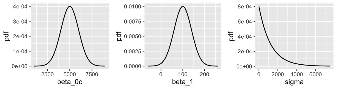

FIGURE 9.4: Prior models for the parameters in the regression analysis of bike ridership, (\(\beta_{0c}\), \(\beta_1\), \(\sigma\)).

Plugging our tuned priors into (9.6), the Bayesian regression model of ridership (\(Y\)) by temperature (\(X\)) is specified as follows:

\[\begin{equation} \begin{split} Y_i | \beta_0, \beta_1, \sigma & \stackrel{ind}{\sim} N\left(\mu_i, \sigma^2\right) \;\; \text{ with } \;\; \mu_i = \beta_0 + \beta_1X_i \\ \beta_{0c} & \sim N\left(5000, 1000^2 \right) \\ \beta_1 & \sim N\left(100, 40^2 \right) \\ \sigma & \sim \text{Exp}(0.0008) .\\ \end{split} \tag{9.7} \end{equation}\]

Since our model utilizes independent priors, we separately processed our prior information on \(\beta_0\), \(\beta_1\), and \(\sigma\) above. Yet we want to make sure that, when combined, these priors actually reflect our current understanding of the relationship between ridership and temperature. To this end, Figure 9.5 presents various scenarios simulated from our prior models.⁴⁸ The 200 prior model lines, \(\beta_0 + \beta_1 X\) (left), do indeed capture our prior understanding that ridership increases with temperature and tends to be around 5000 on average temperature days. The variability in these lines also adequately reflects our overall uncertainty about this association. Next, at right are four ridership datasets simulated from the Normal data model (9.3) using four prior plausible sets of \((\beta_0,\beta_1,\sigma)\) values. If our prior models are reasonable, then data simulated from these models should be consistent with ridership data we’d actually expect to see in practice. That’s indeed the case here. The rate of increase in ridership with temperature, the baseline ridership, and the variability in ridership are consistent with our prior assumptions.

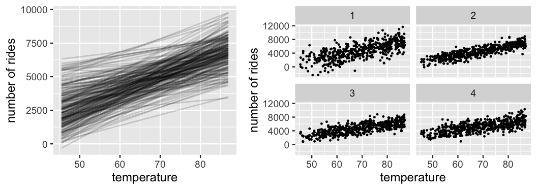
FIGURE 9.5: Simulated scenarios under the prior models of \(\beta_0\), \(\beta_1\), and \(\sigma\). At left are 200 prior plausible model lines, \(\beta_0 + \beta_1 X\). At right are 4 prior plausible datasets.

9.3 Posterior simulation

In the next step of our Bayesian analysis, let’s update our prior understanding of the relationship between ridership and temperature using data. The bikes data in the bayesrules package is a subset of the Bike Sharing dataset made available on the UCI Machine Learning Repository (2017) by Fanaee-T and Gama (2014).⁴⁹ For each of 500 days in the study, bikes contains the number of rides taken and a measure of what the temperature felt like when incorporating factors such as humidity (temp_feel). A scatterplot of rides by temp_feel supports our prior assumption of a positive linear relationship between the two, i.e., \(\mu = \beta_0 + \beta_1 X\) with \(\beta_1 > 0\). Further, the strength of this relationship appears moderate – \(\sigma\) is neither small nor big.

# Load and plot data
data(bikes)
ggplot(bikes, aes(x = temp_feel, y = rides)) + 
  geom_point(size = 0.5) + 
  geom_smooth(method = "lm", se = FALSE)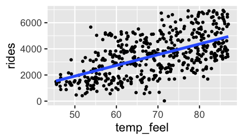

FIGURE 9.6: A scatterplot of ridership vs temperature on 500 different days.

We can now combine the information from this data with that from the prior to build a posterior model for parameters \((\beta_0, \beta_1, \sigma)\). Our inclination here is to jump straight to an MCMC simulation of this posterior, without even attempting to specify this model mathematically. However, we’ll pause long enough to convince you that simulation is the reasonable choice here. Consider the general Bayesian simple regression model (9.6) and let \(\vec{y} = (y_1,y_2,...,y_{n})\) denote a collection of \(n\) observed \(Y\) values. Assuming that the regression parameters are independent, their joint prior pdf is the product of their marginal pdfs which, in turn, are defined by their respective Normal and Exponential prior models:

\[f(\beta_0, \beta_1, \sigma) = f(\beta_0) f(\beta_1) f(\sigma) .\]

Further, the likelihood function of the parameters given the independent data \(\vec{y}\) is defined by the joint pdf of \(\vec{y}\) which, in turn, is the product of the marginal pdfs defined by the Normal data structure (9.3):

\[L(\beta_0, \beta_1, \sigma | \vec{y}) = f(\vec{y}|\beta_0, \beta_1, \sigma) = \prod_{i=1}^{n}f(y_i|\beta_0, \beta_1, \sigma) .\]

Thus, building the posterior model of \((\beta_0, \beta_1, \sigma)\) would require us to specify the joint posterior pdf

\[f(\beta_0,\beta_1,\sigma \; | \; \vec{y}) \propto \text{prior} \cdot \text{likelihood} = f(\beta_0) f(\beta_1) f(\sigma) \cdot \left[\prod_{i=1}^{n}f(y_i | \beta_0, \beta_1, \sigma) \right] . \]

If you went through the tedious work of plugging in the formulas for the \(3 + n\) pdfs in the product above, you wouldn’t discover a familiar structure. Thus, if you really wanted to specify the posterior pdf, you’d need to calculate the normalizing constant. But you might not get far – the constant which guarantees that \(f(\beta_0,\beta_1,\sigma | \vec{y})\) integrates to 1 across all possible sets of \((\beta_0,\beta_1,\sigma)\) is a triple integral of our complicated product:

\[\begin{split} f(\beta_0,\beta_1,\sigma \; | \; \vec{y}) & = \frac{\text{prior} \cdot \text{likelihood}}{ \int \text{prior} \cdot \text{likelihood}} \\ & = \frac{f(\beta_0) f(\beta_1) f(\sigma) \cdot \left[\prod_{i=1}^{n}f(y_i|\beta_0, \beta_1, \sigma) \right]} {\int\int\int f(\beta_0) f(\beta_1) f(\sigma) \cdot \left[\prod_{i=1}^{n}f(y_i|\beta_0, \beta_1, \sigma) \right] d\beta_0 d\beta_1 d\sigma} \\ \end{split}\]

Let’s not. Instead, we can utilize Markov chain Monte Carlo simulation techniques to approximate the posterior.

9.3.1 Simulation via rstanarm

In Chapter 6, our MCMC approximation process unfolded in two steps using the rstan package: first define and then simulate the model using rstan syntax. Not only can this two-step process get more and more complicated as our Bayesian models get more and more sophisticated, it’s not always unnecessary. The rstanarm package (Gabry and Goodrich 2020c) tailors the power of rstan to applied regression models (arm). As such, it contains one-stop functions for simulating a broad set of pre-defined Bayesian regression models, i.e., no need for step 1! For example, to simulate our Normal Bayesian linear regression model of rides by temp_feel, we can utilize the stan_glm() function, which applies to the wider family of generalized linear regression models (glm):

bike_model <- stan_glm(rides ~ temp_feel, data = bikes,
                       family = gaussian,
                       prior_intercept = normal(5000, 1000),
                       prior = normal(100, 40), 
                       prior_aux = exponential(0.0008),
                       chains = 4, iter = 5000*2, seed = 84735)

The syntax above is common to the other rstanarm models we’ll see in this book and looks more intimidating than it is. In general, stan_glm() requires three types of information:

• Data information
  The first three stan_glm() arguments specify the structure of our data: we want to model ridership by temperature (rides ~ temp_feel) using data = bikes and assuming a Normal data model, aka family = gaussian.

• Prior information
  The prior_intercept, prior, and prior_aux arguments specify the priors of \(\beta_{0c}\), \(\beta_1\), and \(\sigma\), respectively. These match the priors defined by (9.7).

• Markov chain information
  The remaining arguments specify the structure of our MCMC simulation: the number of Markov chains to run, the length or number of iterations of each chain, and the random number seed to use.

After tossing out the first half of Markov chain values from the learning or burn-in phase, the stan_glm() simulation produces four parallel chains of length 5000 for each model parameter: \(\left\lbrace \beta_0^{(1)}, \beta_0^{(2)}, \ldots, \beta_0^{(5000)} \right\rbrace\), \(\left\lbrace \beta_1^{(1)}, \beta_1^{(2)}, \ldots, \beta_1^{(5000)} \right\rbrace\), and \(\left\lbrace \sigma_0^{(1)}, \sigma_0^{(2)}, \ldots, \sigma_0^{(5000)} \right\rbrace\). These are stored as (Intercept), temp_feel, and sigma, respectively. Some quick diagnostics indicate that these chains are trustworthy. The effective sample size ratios are slightly above 1 and the R-hat values are very close to 1, indicating that the chains are stable, mixing quickly, and behaving much like an independent sample.

# Effective sample size ratio and Rhat
neff_ratio(bike_model)
(Intercept)   temp_feel       sigma 
      1.042       1.037       1.004 
rhat(bike_model)
(Intercept)   temp_feel       sigma 
     0.9999      0.9999      1.0000 

We come to similar conclusions from the trace and density plots (Figure ??).

# Trace plots of parallel chains
mcmc_trace(bike_model, size = 0.1)

# Density plots of parallel chains
mcmc_dens_overlay(bike_model)

9.3.2 Optional: Simulation via rstan

Though the rstanarm package includes shortcut functions for the types of models we’ll be building in this book, you might be curious how the rstan techniques from Chapter 6 scale up to Normal regression, and hence other models beyond the scope of Unit 1. If you are curious, please read on. Otherwise, please skip to the next section.

In rstanarm, the use of stan_glm() with family = gaussian both defined the exact structure of our Bayesian model and simulated the corresponding posterior. In rstan we have to separately define and simulate our model, steps 1 and 2. Consider the important pieces of information we must communicate in step 1:

• data: The data on variables Y and X, rides and temperature, will be vectors of length n.
• parameters: Our two regression coefficients beta0 and beta1 (\(\beta_0\) and \(\beta_1\)) can both be any real number whereas the standard deviation parameter standard deviation parameter sigma (\(\sigma\)) must be non-negative.
• model: The data model of Y is normal with mean beta0 + beta1 * X and standard deviation sigma. Further, with the exception of beta0, the priors are similar to those in our stan_glm() syntax. Using rstan, we must directly express our prior understanding of the intercept \(\beta_0\), not the centered intercept \(\beta_{0c}\). In this case, we can extend our prior understanding that there are typically 5000 riders on a 70-degree day, to there being -2000 hypothetical riders on a 0-degree day (Figure 9.3).

# STEP 1: DEFINE the model
stan_bike_model <- "
  data {
    int<lower = 0> n;
    vector[n] Y;
    vector[n] X;
  }
  parameters {
    real beta0;
    real beta1;
    real<lower = 0> sigma;
  }
  model {
    Y ~ normal(beta0 + beta1 * X, sigma);
    beta0 ~ normal(-2000, 1000);
    beta1 ~ normal(100, 40);
    sigma ~ exponential(0.0008);
  }
"

In step 2, we simulate the posterior model of \((\beta_0,\beta_1,\sigma)\) using the stan() function. The only difference here from the models we simulated in Chapter 6 is that we have more pieces of data: data on sample size n, response variable Y, and predictor X:

# STEP 2: SIMULATE the posterior
stan_bike_sim <- 
  stan(model_code = stan_bike_model, 
       data = list(n = nrow(bikes), Y = bikes$rides, X = bikes$temp_feel), 
       chains = 4, iter = 5000*2, seed = 84735)

Though they ultimately contain similar information about the approximate posterior model of \((\beta_0, \beta_1, \sigma)\), the structures of the rstan stan_bike_sim object and rstanarm bike_model object slightly differ. And now that we’ve made the connection between rstan and rstanarm here, moving forward we’ll focus on the rstanarm shortcuts and their output. Should you wish to learn more about rstan, the Stan development team provides an excellent resource (Stan development team 2019).

9.4 Interpreting the posterior

We’ve now successfully simulated the posterior Normal regression model of bikeshare ridership by temperature. So what does it all mean?! The mcmc_dens_overlay() plot in Figure ?? allows us to visualize and examine the approximate posterior models for each of the regression parameters \(\beta_0\), \(\beta_1\), and \(\sigma\). Posterior summary statistics, calculated via the tidy() function in the broom.mixed package, provide complementary numerical summaries. Since our Normal regression model has more than one parameter, we must specify the “effects” or parameters of interest. Here, we summarize both the fixed regression coefficients, \(\beta_0\) and \(\beta_1\), and the aux (or auxiliary) parameter \(\sigma\):

# Posterior summary statistics
tidy(bike_model, effects = c("fixed", "aux"),
     conf.int = TRUE, conf.level = 0.80)
# A tibble: 4 x 5
  term        estimate std.error conf.low conf.high
  <chr>          <dbl>     <dbl>    <dbl>     <dbl>
1 (Intercept)  -2194.     362.    -2656.    -1732. 
2 temp_feel       82.2      5.15     75.6      88.8
3 sigma         1281.      40.7    1231.     1336. 
4 mean_PPD      3487.      80.4    3385.     3591. 

Let’s first focus on the typical relationship between ridership and temperature, \(\mu = \beta_0 + \beta_1 X\). Referring to the tidy() summary, the posterior median relationship is

\[\begin{equation} -2194.24 + 82.16 X . \tag{9.8} \end{equation}\]

That is, for every one degree increase in temperature, we expect ridership to increase by roughly 82 rides. There is, of course, posterior uncertainty in this relationship. For example, the 80% posterior credible interval for \(\beta_1\), (75.6, 88.8), indicates that this slope could range anywhere between 76 and 89. To combine this uncertainty in \(\beta_1\) with that in \(\beta_0\) for a better overall picture of our model, notice that the Markov chain simulations provide 20,000 posterior plausible pairs of \(\beta_0\) and \(\beta_1\) values:

# Store the 4 chains for each parameter in 1 data frame
bike_model_df <- as.data.frame(bike_model)

# Check it out
nrow(bike_model_df)
[1] 20000
head(bike_model_df, 3)
  (Intercept) temp_feel sigma
1       -2657     88.16  1323
2       -2188     83.01  1323
3       -1984     81.54  1363

These pairs provide 20,000 alternative scenarios for the typical relationship between ridership and temperature, \(\beta_0 + \beta_1 X\), and thus capture our overall uncertainty about this relationship. For example, the first pair indicates the plausibility that \(\beta_0 + \beta_1 X\) \(=\) -2657 \(+\) 88.2 \(X\). The second pair has a higher intercept and a smaller slope. Below we plot just 50 of these 20,000 posterior plausible mean models, \(\beta_0^{(i)} + \beta_1^{(i)}X\). This is a multi-step process:

• The add_fitted_draws() function from the tidybayes package (Kay 2021) evaluates 50 posterior plausible relationships, \(\beta_0^{(i)} + \beta_1^{(i)}X\), along the observed range of temperatures \(X\). We encourage you to increase this number – plotting more than 50 lines here just doesn’t print nicely.
• We then plot these 50 model lines, labeled by .draw, on top of the observed data points using ggplot().

# 50 simulated model lines
bikes %>%
  add_fitted_draws(bike_model, n = 50) %>%
  ggplot(aes(x = temp_feel, y = rides)) +
    geom_line(aes(y = .value, group = .draw), alpha = 0.15) + 
    geom_point(data = bikes, size = 0.05)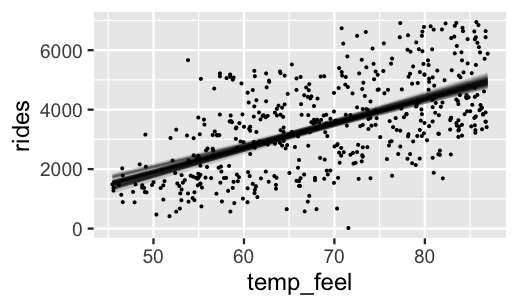

FIGURE 9.7: Model lines constructed from 50 posterior plausible sets of \(\beta_0\) and \(\beta_1\).

Comparing the posterior plausible models in Figure 9.7 to the prior plausible models in Figure 9.5 reveals the evolution in our understanding of ridership. First, the increase in ridership with temperature appears to be less steep than we had anticipated. Further, the posterior plausible models are far less variable, indicating that we’re far more confident about the relationship between ridership and temperature upon observing some data. Once you’ve reflected on the results above, quiz yourself.

Do we have ample posterior evidence that there’s a positive association between ridership and temperature, i.e., that \(\beta_1 > 0\)? Explain.

The answer to the quiz is yes. We can support this answer with three types of evidence.

• Visual evidence
  In our visual examination of 50 posterior plausible scenarios for the relationship between ridership and temperature (Figure 9.7), all exhibited positive associations. A line exhibiting no relationship (\(\beta_1 = 0\)) would stick out like a sore thumb.

• Numerical evidence from the posterior credible interval
  More rigorously, the 80% credible interval for \(\beta_1\) in the above tidy() summary, (75.6, 88.8), lies entirely and well above 0.

• Numerical evidence from a posterior probability
  To add one more unnecessary piece of evidence to the pile, a quick tabulation approximates that there’s almost certainly a positive association, \(P(\beta_1 > 0 \; | \; \vec{y}) \approx 1\). Of our 20,000 Markov chain values of \(\beta_1\), zero are positive.

  # Tabulate the beta_1 values that exceed 0
  bike_model_df %>% 
    mutate(exceeds_0 = temp_feel > 0) %>% 
    tabyl(exceeds_0)
   exceeds_0     n percent
        TRUE 20000       1

Finally, let’s examine the posterior results for \(\sigma\), the degree to which ridership varies on days of the same temperature. Above we estimated that \(\sigma\) has a posterior median of 1281 and an 80% credible interval (1231, 1336). Thus, on average, we can expect the observed ridership on a given day to fall 1281 rides from the average ridership on days of the same temperature. Figure 9.7 adds some context, presenting four simulated sets of ridership data under four posterior plausible values of \(\sigma\). At least visually, these plots exhibit similarly moderate relationships, indicating relative posterior certainty about the strength in the relationship between ridership and temperature. The syntax here is quite similar to that used for plotting the plausible regression lines \(\beta_0 + \beta_1 X\) in Figure 9.7. The main difference is that we’ve replaced add_fitted_draws with add_predicted_draws.

# Simulate four sets of data
bikes %>%
  add_predicted_draws(bike_model, n = 4) %>%
  ggplot(aes(x = temp_feel, y = rides)) +
    geom_point(aes(y = .prediction, group = .draw), size = 0.2) + 
    facet_wrap(~ .draw)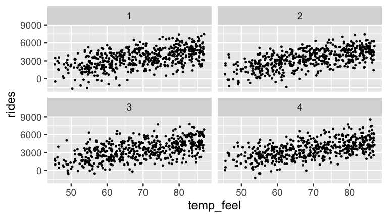

FIGURE 9.8: Four datasets simulated from the posterior models of \(\beta_0\), \(\beta_1\), and \(\sigma\).

9.5 Posterior prediction

Our above examination of the regression parameters illuminates the relationship between ridership and temperature. Beyond building such insight, a common goal of regression analysis is to use our model to make predictions.

Suppose a weather report indicates that tomorrow will be a 75-degree day in D.C. What’s your posterior guess of the number of riders that Capital Bikeshare should anticipate?

Your natural first crack at this question might be to plug the 75-degree temperature into the posterior median model (9.8). Thus, we expect that there will be 3968 riders tomorrow:

\[-2194.24 + 82.16*75 = 3967.76 .\]

BUT, recall from Section 8.4.3 that this singular prediction ignores two potential sources of variability:

• Sampling variability in the data
  The observed ridership outcomes, \(Y\), typically deviate from the model line. That is, we don’t expect every 75-degree day to have the same exact number of rides.

• Posterior variability in parameters \((\beta_0, \beta_1, \sigma)\)
  The posterior median model is merely the center in a range of plausible model lines \(\beta_0 + \beta_1 X\) (Figure 9.7). We should consider this entire range as well as that in \(\sigma\), the degree to which observations might deviate from the model lines.

The posterior predictive model of a new data point \(Y_{\text{new}}\) accounts for both sources of variability. Specifically, the posterior predictive pdf captures the overall chance of observing \(Y_{\text{new}} = y_{\text{new}}\) by weighting the chance of this outcome under any set of possible parameters (\(f(y_{new} | \beta_0,\beta_1,\sigma)\)) by the posterior plausibility of these parameters (\(f(\beta_0,\beta_1,\sigma|\vec{y})\)). Mathematically speaking:

\[f\left(y_{\text{new}} | \vec{y}\right) = \int\int\int f\left(y_{new} | \beta_0,\beta_1,\sigma\right) f(\beta_0,\beta_1,\sigma|\vec{y}) d\beta_0 d\beta_1 d\sigma .\]

Now, we don’t actually have a nice, tidy formula for the posterior pdf of our regression parameters, \(f(\beta_0,\beta_1,\sigma|\vec{y})\), and thus can’t get a nice tidy formula for the posterior predictive pdf \(f\left(y_{\text{new}} | \vec{y}\right)\). What we do have is 20,000 sets of parameters in the Markov chain \(\left(\beta_0^{(i)},\beta_1^{(i)},\sigma^{(i)}\right)\). We can then approximate the posterior predictive model for \(Y_{\text{new}}\) at \(X = 75\) by simulating a ridership prediction from the Normal model evaluated each parameter set:

\[Y_{\text{new}}^{(i)} | \beta_0, \beta_1, \sigma \; \sim \; N\left(\mu^{(i)}, \left(\sigma^{(i)}\right)^2\right) \;\; \text{ with } \;\; \mu^{(i)} = \beta_0^{(i)} + \beta_1^{(i)} \cdot 75.\]

Thus, each of the 20,000 parameter sets in our Markov chain (left) produces a unique prediction (right):

\[\left[ \begin{array}{lll} \beta_0^{(1)} & \beta_1^{(1)} & \sigma^{(1)} \\ \beta_0^{(2)} & \beta_1^{(2)} & \sigma^{(2)} \\ \vdots & \vdots & \vdots \\ \beta_0^{(20000)} & \beta_1^{(20000)} & \sigma^{(20000)} \\ \end{array} \right] \;\; \longrightarrow \;\; \left[ \begin{array}{l} Y_{\text{new}}^{(1)} \\ Y_{\text{new}}^{(2)} \\ \vdots \\ Y_{\text{new}}^{(20000)} \\ \end{array} \right]\]

The resulting collection of 20,000 predictions, \(\left\lbrace Y_{\text{new}}^{(1)}, Y_{\text{new}}^{(2)}, \ldots, Y_{\text{new}}^{(20000)} \right\rbrace\), approximates the posterior predictive model of ridership \(Y\) on 75-degree days. We will obtain this approximation both “by hand,” which helps us build some powerful intuition, and using shortcut R functions.

9.5.1 Building a posterior predictive model

To really connect with the concepts, let’s start by approximating posterior predictive models without the use of a shortcut function. To do so, we’ll simulate 20,000 predictions of ridership on a 75-degree day, \(\left\lbrace Y_{\text{new}}^{(1)}, Y_{\text{new}}^{(2)}, \ldots, Y_{\text{new}}^{(20000)} \right\rbrace\), one from each parameter set in bike_model_df. Let’s start small with just the first posterior plausible parameter set:

first_set <- head(bike_model_df, 1)
first_set
  (Intercept) temp_feel sigma
1       -2657     88.16  1323

Under this particular scenario, \(\left(\beta_0^{(1)}, \beta_1^{(1)}, \sigma^{(1)}\right) = (-2657, 88.16, 1323)\), the average ridership at a given temperature is defined by

\[\mu = \beta_0^{(1)} + \beta_1^{(1)} X = -2657 + 88.16X .\]

As such, we’d expect an average of \(\mu = 3955\) riders on a 75-degree day:

mu <- first_set$`(Intercept)` + first_set$temp_feel * 75
mu
[1] 3955

To capture the sampling variability around this average, i.e., the fact that not all 75-degree days have the same ridership, we can simulate our first official prediction \(Y_{\text{new}}^{(1)}\) by taking a random draw from the Normal model specified by this first parameter set:

\[Y_{\text{new}}^{(1)} | \beta_0, \beta_1, \sigma \; \sim \; N\left(3955, 1323^2\right) .\]

Taking a draw from this model using rnorm(), we happen to observe an above average 4838 rides on the 75-degree day:

set.seed(84735)
y_new <- rnorm(1, mean = mu, sd = first_set$sigma)
y_new
[1] 4838

Now let’s do this 19,999 more times. That is, let’s follow the same two-step process to simulate a prediction of ridership from each of the 20,000 sets of regression parameters \(i\) in bike_model_df: (1) calculate the average ridership on 75-degree days, \(\mu^{(i)} = \beta_0^{(i)} + \beta_1^{(i)}\cdot 75\); then (2) sample from the Normal model centered at this average with standard deviation \(\sigma^{(i)}\):

# Predict rides for each parameter set in the chain
set.seed(84735)
predict_75 <- bike_model_df %>% 
  mutate(mu = `(Intercept)` + temp_feel*75,
         y_new = rnorm(20000, mean = mu, sd = sigma))

The first 3 sets of average ridership (mu) and predicted ridership on a specific day (y_new) are shown here along with the first 3 posterior plausible parameter sets from which they were generated ((Intercept), temp_feel, sigma):

head(predict_75, 3)
  (Intercept) temp_feel sigma   mu y_new
1       -2657     88.16  1323 3955  4838
2       -2188     83.01  1323 4038  3874
3       -1984     81.54  1363 4132  5196

Whereas the collection of 20,000 mu values approximates the posterior model for the typical ridership on 75-degree days, \(\mu = \beta_0 + \beta_1 * 75\), the 20,000 y_new values approximate the posterior predictive model of ridership for tomorrow, an individual 75-degree day,

\[Y_{\text{new}} | \beta_0, \beta_1, \sigma \; \sim \; N\left(\mu, \sigma^2\right) \;\; \text{ with } \;\; \mu = \beta_0 + \beta_1 \cdot 75 .\]

In the plots of these two posterior models (Figure 9.9), you’ll immediately pick up the fact that, though they’re centered at roughly the same value, the posterior predictive model for mu is much narrower than that of y_new. Specifically, the 95% credible interval for the typical number of rides on a 75-degree day, \(\mu\), ranges from 3843 to 4095. In contrast, the 95% posterior prediction interval for the number of rides tomorrow has a much wider range from 1500 to 6482.

# Construct 80% posterior credible intervals
predict_75 %>% 
  summarize(lower_mu = quantile(mu, 0.025),
            upper_mu = quantile(mu, 0.975),
            lower_new = quantile(y_new, 0.025),
            upper_new = quantile(y_new, 0.975))
  lower_mu upper_mu lower_new upper_new
1     3843     4095      1500      6482

# Plot the posterior model of the typical ridership on 75 degree days
ggplot(predict_75, aes(x = mu)) + 
  geom_density()

# Plot the posterior predictive model of tomorrow's ridership
ggplot(predict_75, aes(x = y_new)) + 
  geom_density()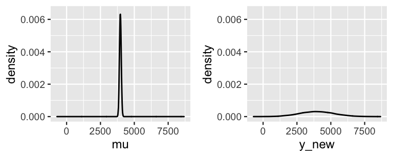

FIGURE 9.9: The posterior model of \(\mu\), the typical ridership on a 75-degree day (left), and the posterior predictive model of the ridership tomorrow, a specific 75-degree day (right).

These two 95% intervals are represented on a scatterplot of the observed data (Figure 9.10), clarifying that the posterior model for \(\mu\) merely captures the uncertainty in the average ridership on all \(X = 75\)-degree days. Since there is so little uncertainty about this average, this interval visually appears like a wee dot! In contrast, the posterior predictive model for the number of rides tomorrow (a specific day) accounts for not only the average ridership on a 75-degree day, but the individual variability from this average. The punchline? There’s more accuracy in anticipating the average behavior across multiple data points than the unique behavior of a single data point.

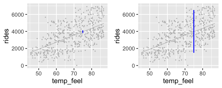
FIGURE 9.10: 95% posterior credible intervals (blue) for the average ridership on 75-degree days (left) and the predicted ridership for tomorrow, an individual 75-degree day (right).

9.5.2 Posterior prediction with rstanarm

Simulating the posterior predictive model from scratch allowed you to really connect with the concept, but moving forward we can utilize the posterior_predict() function in the rstanarm package:

# Simulate a set of predictions
set.seed(84735)
shortcut_prediction <- 
  posterior_predict(bike_model, newdata = data.frame(temp_feel = 75))

The shortcut_prediction object contains 20,000 predictions of ridership on 75-degree days. We can both visualize and summarize the corresponding (approximate) posterior predictive model using our usual tricks. The results are equivalent to those we constructed from scratch above:

# Construct a 95% posterior credible interval
posterior_interval(shortcut_prediction, prob = 0.95)
  2.5% 97.5%
1 1500  6482

# Plot the approximate predictive model
mcmc_dens(shortcut_prediction) + 
  xlab("predicted ridership on a 75 degree day")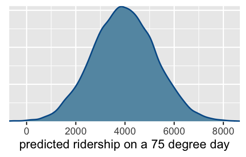

FIGURE 9.11: Posterior predictive model of ridership on a 75-degree day.

9.6 Sequential regression modeling

Our analysis above spotlighted the newest concept of the book: modeling the relationship between two variables \(Y\) and \(X\). Yet our Bayesian thinking, second nature by now, provided the foundation for this analysis. Here, let’s consider another attractive feature of Bayesian thinking, sequentiality, in the context of regression modeling (Chapter 4). Above we analyzed the complete bikes data that spanned 500 different days, arranged by date:

bikes %>% 
  select(date, temp_feel, rides) %>% 
  head(3)
        date temp_feel rides
1 2011-01-01     64.73   654
2 2011-01-03     49.05  1229
3 2011-01-04     51.09  1454

Suppose instead that we were given access to this data in bits and pieces, as it became available: after the first 30 days of data collection, then again after the first 60 days, and finally after all 500 days.

phase_1 <- bikes[1:30, ]
phase_2 <- bikes[1:60, ]
phase_3 <- bikes

After each data collection phase, we can re-simulate the posterior model by plugging in the accumulated data (phase_1, phase_2, or phase_3):

my_model <- stan_glm(rides ~ temp_feel, data = ___, family = gaussian, 
                     prior_intercept = normal(5000, 1000),
                     prior = normal(100, 40), 
                     prior_aux = exponential(0.0008),
                     chains = 4, iter = 5000*2, seed = 84735)

Figure 9.12 displays the posterior models for the temperature coefficient \(\beta_1\) after each phase of data collection, and thus the evolution in our understanding of the relationship between ridership and temperature. What started in Phase 1 as a vague understanding that there might be no relationship between ridership and temperature (\(\beta_1\) values near 0 are plausible), evolved into clear understanding by Phase 3 that ridership tends to increase by roughly 80 rides per one degree increase in temperature.

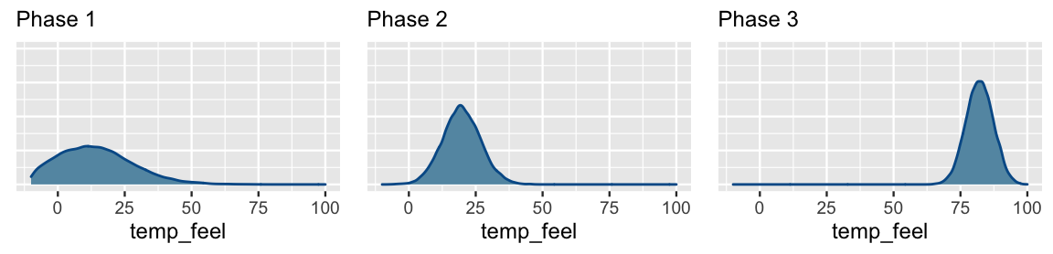
FIGURE 9.12: Approximate posterior models for the temperature coefficient \(\beta_1\) after three phases of data collection.

Figure 9.13 provides more insight into this evolution, displaying the accumulated data and 100 posterior plausible models at each phase in our analysis. Having observed only 30 data points, the Phase 1 posterior models are all over the map. Further, since these 30 data points happened to land on cold days in the winter, our Phase 1 information did not yet reveal that ridership tends to increase on warmer days. Over Phases 2 and 3, we not only gathered more data, but data which allows us to examine the ridership across the full spectrum of temperatures in Washington, D.C. By the end of Phase 3, we have great posterior certainty of the positive association between these two variables. Again, this kind of evolution in our understanding is how learning, science, progress happen. Knowledge is built up, piece by piece, over time.

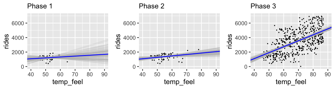
FIGURE 9.13: 100 simulated posterior median models of ridership vs temperature after three phases of data collection.

9.7 Using default rstanarm priors

It’s not always the case that we’ll have such strong prior information as we did in the bike analysis. As such, we’ll want to tune our prior models to reflect this great uncertainty. To this end, we recommend utilizing the default priors in the rstanarm package. The default tuning for our Bayesian regression model of Capital Bikeshare ridership (\(Y\)) by temperature (\(X\)) is shown below (9.9). The only holdover from the original priors (9.7) is our assumption that the average ridership tends to be around 5000 on average temperature days. Even when we don’t have strong prior information, we often have a sense of the baseline.

\[\begin{equation} \begin{split} Y_i | \beta_0, \beta_1, \sigma & \stackrel{ind}{\sim} N\left(\mu_i, \sigma^2\right) \;\; \text{ with } \;\; \mu_i = \beta_0 + \beta_1X_i \\ \beta_{0c} & \sim N\left(5000, 3937^2 \right) \\ \beta_1 & \sim N\left(0, 351^2 \right) \\ \sigma & \sim \text{Exp}(0.00064) .\\ \end{split} \tag{9.9} \end{equation}\]

The prior tunings here might seem bizarrely specific. We’ll explain. When we don’t have specific prior information, we can utilize rstanarm’s defaults through the following syntax. (We could also omit all prior information whatsoever, in which case stan_glm() would automatically assign priors. However, given different versions of the software, the results may not be reproducible.)

bike_model_default <- stan_glm(
  rides ~ temp_feel, data = bikes, 
  family = gaussian,
  prior_intercept = normal(5000, 2.5, autoscale = TRUE),
  prior = normal(0, 2.5, autoscale = TRUE), 
  prior_aux = exponential(1, autoscale = TRUE),
  chains = 4, iter = 5000*2, seed = 84735)

This syntax specifies the following priors: \(\beta_{0c} \sim N(5000, 2.5^2)\), \(\beta_1 \sim N(0, 2.5^2)\), and \(\sigma \sim \text{Exp}(1)\). With a twist. Consider the priors for \(\beta_{0c}\) and \(\beta_1\). Assuming we have a weak prior understanding of these parameters, and hence their scales, we’re not really sure whether a standard deviation of 2.5 is relatively small or relatively large. Thus, we’re not really sure if these priors are more specific than we want them to be. This is why we also set autoscale = TRUE. By doing so, stan_glm() adjusts or scales our default priors to optimize the study of parameters which have different scales.⁵⁰ These Adjusted priors are specified by the prior_summary() function and match our reported model formulation (9.9):

prior_summary(bike_model_default)
Priors for model 'bike_model_default' 
------
Intercept (after predictors centered)
  Specified prior:
    ~ normal(location = 5000, scale = 2.5)
  Adjusted prior:
    ~ normal(location = 5000, scale = 3937)

Coefficients
  Specified prior:
    ~ normal(location = 0, scale = 2.5)
  Adjusted prior:
    ~ normal(location = 0, scale = 351)

Auxiliary (sigma)
  Specified prior:
    ~ exponential(rate = 1)
  Adjusted prior:
    ~ exponential(rate = 0.00064)
------
See help('prior_summary.stanreg') for more details

In this scaling process, rstanarm seeks to identify weakly informative priors (Gabry and Goodrich 2020b). The idea is similar to vague priors: weakly informative priors reflect general prior uncertainty about the model parameters. However, whereas a vague prior might be so vague that it puts weight on non-sensible parameter values (e.g., \(\beta_1\) values that assume ridership could increase by 1 billion rides for every one degree increase in temperature), weakly informative priors are a bit more focused. They reflect general prior uncertainty across a range of sensible parameter values. As such, weakly informative priors foster computationally efficient posterior simulation since the chains don’t have to waste time exploring non-sensible parameter values.

There’s also a catch. Weakly informative priors are tuned to identify “sensible” parameter values by considering the scales of our data, here ridership and temperature. Though it seems odd to tune priors using data, the process merely takes into account the scales of the variables (e.g., what are temperatures like in D.C.? what’s the variability in ridership from day to day?). It does not consider the relationship among these variables.

Let’s see how these weakly informative priors compare to our original informed priors. Instead of starting from scratch, to simulate our new priors, we update() the bike_model_default with prior_PD = TRUE, thereby indicating we’re interested in the prior not posterior models of \((\beta_0,\beta_1,\sigma)\).

# Perform a prior simulation 
bike_default_priors <- update(bike_model_default, prior_PD = TRUE)

We then plot 200 plausible model lines (\(\beta_0 + \beta_1 X\)) and 4 datasets simulated under the weakly informative priors using the add_fitted_draws() and add_predicted_draws() functions (Figure 9.14). In contrast to the original priors (Figure 9.5), the weakly informative priors in Figure 9.14 reflect much greater uncertainty about the relationship between ridership and temperature. As the Normal prior for \(\beta_1\) is centered at 0, the model lines indicate that the association between ridership and temperature might be positive (\(\beta_1 > 0\)), non-existent (\(\beta_1 = 0\)), or negative (\(\beta_1 < 0\)). Some of the simulated data points even include negative ridership values! Further, the simulated datasets reflect our uncertainty about whether the relationship is strong (with \(\sigma\) near 0) or weak (with large \(\sigma\)). Yet, by utilizing weakly informative priors instead of totally vague priors, our prior uncertainty is still in the right ballpark. Our priors focus on ridership being in the thousands (reasonable), not in the millions or billions (unreasonable for a city of Washington D.C.’s size).

# 200 prior model lines
bikes %>%
  add_fitted_draws(bike_default_priors, n = 200) %>%
  ggplot(aes(x = temp_feel, y = rides)) +
    geom_line(aes(y = .value, group = .draw), alpha = 0.15)

# 4 prior simulated datasets
set.seed(3)
bikes %>%
  add_predicted_draws(bike_default_priors, n = 4) %>%
  ggplot(aes(x = temp_feel, y = rides)) +
    geom_point(aes(y = .prediction, group = .draw)) + 
    facet_wrap(~ .draw)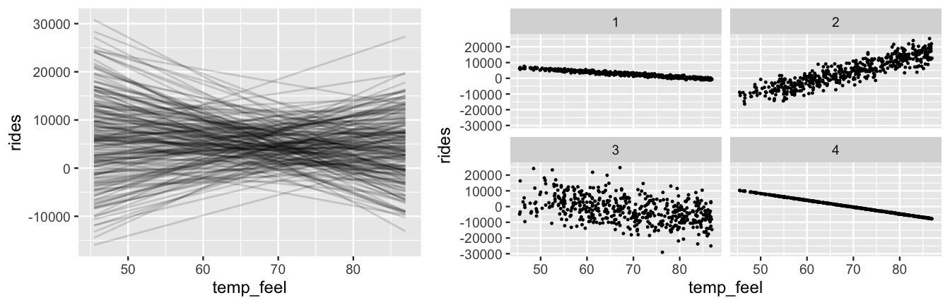

FIGURE 9.14: Simulated scenarios under the default prior models of \(\beta_0\), \(\beta_1\), and \(\sigma\). At left are 200 prior plausible model lines, \(\beta_0 + \beta_1 x\). At right are 4 prior plausible datasets.

Default vs non-default priors

There are pros and cons to utilizing the default priors in rstanarm. In terms of drawbacks, weakly informative priors are tuned with information from the data (through a fairly minor consideration of scale). But on the plus side:

• Unless we have strong prior information, utilizing the defaults will typically lead to more stable simulation results than if we tried tuning our own vague priors.
• The defaults can help us get up and running with Bayesian modeling. In future chapters, we’ll often utilize the defaults in order to focus on the new modeling concepts.

9.8 You’re not done yet!

Taken alone, Chapter 9 is quite dangerous! Thus, far you’ve explored how to build, simulate, and interpret a simple Bayesian Normal regression model. The next crucial step in any analysis is to ask: but is this a good model? This question is deserving of its own chapter. Thus, we strongly encourage you to review Chapter 10 before applying what you’ve learned here.

9.9 Chapter summary

In Chapter 9 you explored how to build a Bayesian simple Normal regression model of a quantitative response variable \(Y\) by a quantitative predictor variable \(X\). We can view this model as an extension of the Normal-Normal model from Chapter 5, where we replace the global mean \(\mu\) by the local mean \(\beta_0 + \beta_1 X\) which incorporates the linear dependence of \(Y\) on \(X\):

\[\begin{split} Y_i | \mu & \stackrel{ind}{\sim} N(\mu, \sigma^2)\\ \mu & \sim N(\theta, \tau^2)\\ & \\ & \\ \end{split} \;\; \Rightarrow \;\; \begin{split} Y_i|\beta_0,\beta_1,\sigma & \stackrel{ind}{\sim} N(\mu_i, \; \sigma^2) \;\; \text{ with } \;\; \mu_i = \beta_0 + \beta_1 X_i \\ \beta_0 & \sim N\left(m_0, s_0^2 \right) \\ \beta_1 & \sim N\left(m_1, s_1^2 \right) \\ \sigma & \sim \text{Exp}(l)\\ \end{split}\]

This extension introduces three unknown model parameters, \((\beta_0, \beta_1, \sigma)\), an added complexity which requires Markov chain Monte Carlo simulation techniques to approximate the posterior model of these parameters. This simulation output can then be used to summarize our posterior understanding of the relationship between \(Y\) and \(X\).

9.10 Exercises

9.10.1 Conceptual exercises

Exercise 9.1 (Normal regression priors) For the Normal regression model (9.6) with \(Y_i|\beta_0, \beta_1, \sigma \sim N(\mu_i, \sigma)\) where \(\mu_i = \beta_0 + \beta_1X_i\), we utilized Normal priors for \(\beta_0, \beta_1\) and an Exponential prior on \(\sigma\).

1. Why is a Normal prior a reasonable choice for \(\beta_0\) and \(\beta_1\)?
2. Why isn’t a Normal prior a reasonable choice for \(\sigma\)?
3. What’s the difference between weakly informative and vague priors?

Exercise 9.2 (Identify the variable) Identify the response variable (\(Y\)) and predictor variable (\(X\)) in each given relationship of interest.

1. We want to use a person’s arm length to understand their height.
2. We want to predict a person’s carbon footprint (in annual CO\(_2\) emissions) with the distance between their home and work.
3. We want to understand how a child’s vocabulary level might increase with age.
4. We want to use information about a person’s sleep habits to predict their reaction time.

Exercise 9.3 (Interpreting coefficients) In each situation below, suppose that the typical relationship between the given response variable \(Y\) and predictor \(X\) can be described by \(\beta_0 + \beta_1 X\). Interpret the meaning of \(\beta_0\) and \(\beta_1\) and indicate whether your prior understanding suggests that \(\beta_1\) is negative or positive.

1. \(Y\) = height in cm of a baby kangaroo, \(X\) = its age in months
2. \(Y\) = a data scientist’s number of GitHub followers, \(X\) = their number of GitHub commits in the past week
3. \(Y\) = number of visitors to a local park on a given day, \(X\) = rainfall in inches on that day
4. \(Y\) = the daily hours of Netflix that a person watches, \(X\) = the typical number of hours that they sleep

Exercise 9.4 (Deviation from the average) Consider the Normal regression model (9.6). Explain in one or two sentences, in a way that one of your non-stats friends could understand, how \(\sigma\) is related to the strength of the relationship between a response variable \(Y\) and predictor \(X\).

Exercise 9.5 (Bayesian model building: Part I) A researcher wants to use a person’s age (in years) to predict their annual orange juice consumption (in gallons). Here you’ll build up a relevant Bayesian regression model, step by step.

1. Identify the \(Y\) and \(X\) variables in this study.
2. Use mathematical notation to specify an appropriate structure for the model of data \(Y\) (ignoring \(X\) for now).
3. Rewrite the structure of the data model to incorporate information about predictor \(X\). In doing so, assume there’s a linear relationship between \(Y\) and \(X\).
4. Identify all unknown parameters in your model. For each, indicate the values the parameter can take.
5. Identify and tune suitable prior models for your parameters. Explain your rationale.

Exercise 9.6 (Bayesian model building: Part II) Repeat the above exercise for the following scenario. A researcher wishes to predict tomorrow’s high temperature by today’s high temperature.

Exercise 9.7 (Posterior simulation T/F) Mark each statement about posterior regression simulation as True or False.

1. MCMC provides the exact posterior model of our regression parameters \((\beta_0,\beta_1,\sigma)\).
2. MCMC allows us to avoid complicated mathematical derivations.

Exercise 9.8 (Posterior simulation) For each situation, specify the appropriate stan_glm() syntax for simulating the Normal regression model using 4 chains, each of length 10000. (You won’t actually run any code.)

1. \(X\) = age; \(Y\) = height; dataset name: bunnies
2. \(\text{Clicks}_i | \beta_0, \beta_1, \sigma \sim N\left(\mu_i, \sigma^2\right) \;\; \text{ with } \;\; \mu_i = \beta_0 + \beta_1\text{Snaps}_i\); dataset name: songs.
3. \(\text{Happiness}_i | \beta_0, \beta_1, \sigma \sim N\left(\mu_i, \sigma^2\right) \;\; \text{ with } \;\; \mu_i = \beta_0 + \beta_1\text{Age}_i\); dataset name: dogs.

9.10.2 Applied exercises

Exercise 9.9 (How humid is too humid: model building) Throughout this chapter, we explored how bike ridership fluctuates with temperature. But what about humidity? In the next exercises, you will explore the Normal regression model of rides (\(Y\)) by humidity (\(X\)) using the bikes dataset. Based on past bikeshare analyses, suppose we have the following prior understanding of this relationship:

• On an average humidity day, there are typically around 5000 riders, though this average could be somewhere between 1000 and 9000.

• Ridership tends to decrease as humidity increases. Specifically, for every one percentage point increase in humidity level, ridership tends to decrease by 10 rides, though this average decrease could be anywhere between 0 and 20.

• Ridership is only weakly related to humidity. At any given humidity, ridership will tend to vary with a large standard deviation of 2000 rides.

1. Tune the Normal regression model (9.6) to match our prior understanding. Use careful notation to write out the complete Bayesian structure of this model.
2. To explore our combined prior understanding of the model parameters, simulate the Normal regression prior model with 5 chains run for 8000 iterations each. HINT: You can use the same stan_glm() syntax that you would use to simulate the posterior, but include prior_PD = TRUE.
3. Plot 100 prior plausible model lines (\(\beta_0 + \beta_1 X\)) and 4 datasets simulated under the priors.
4. Describe our overall prior understanding of the relationship between ridership and humidity.

Exercise 9.10 (How humid is too humid: data) With the priors in place, let’s examine the data.

1. Plot and discuss the observed relationship between ridership and humidity in the bikes data.
2. Does simple Normal regression seem to be a reasonable approach to modeling this relationship? Explain.

Exercise 9.11 (How humid is too humid: posterior simulation) We can now simulate our posterior model of the relationship between ridership and humidity, a balance between our prior understanding and the data.

1. Use stan_glm() to simulate the Normal regression posterior model. Do so with 5 chains run for 8000 iterations each. HINT: You can either do this from scratch or update() your prior simulation from Exercise 9.9 using prior_PD = FALSE.
2. Perform and discuss some MCMC diagnostics to determine whether or not we can “trust” these simulation results.
3. Plot 100 posterior model lines for the relationship between ridership and humidity. Compare and contrast these to the prior model lines from Exercise 9.9.

Exercise 9.12 (How humid is too humid: posterior interpretation) Finally, let’s dig deeper into our posterior understanding of the relationship between ridership and humidity.

1. Provide a tidy() summary of your posterior model, including 95% credible intervals.
2. Interpret the posterior median value of the \(\sigma\) parameter.
3. Interpret the 95% posterior credible interval for the humidity coefficient, \(\beta_1\).
4. Do we have ample posterior evidence that there’s a negative association between ridership and humidity? Explain.

Exercise 9.13 (How humid is too humid: prediction) Tomorrow is supposed to be 90% humidity in Washington, D.C. What levels of ridership should we expect?

1. Without using the posterior_predict() shortcut function, simulate two posterior models:
   • the posterior model for the typical number of riders on 90% humidity days; and
   • the posterior predictive model for the number of riders tomorrow.
2. Construct, discuss, and compare density plot visualizations for the two separate posterior models in part a.
3. Calculate and interpret an 80% posterior prediction interval for the number of riders tomorrow.
4. Use posterior_predict() to confirm the results from your posterior predictive model of tomorrow’s ridership.

Exercise 9.14 (On your own: Part I) Temperature and humidity aren’t the only possible weather factors in ridership. Let’s explore the relationship between ridership (\(Y\)) and windspeed (\(X\)).

1. Describe your own prior understanding of the relationship between ridership and wind speed.
2. Tune the Normal regression model (9.6) to match your prior understanding. Use careful notation to write out the complete Bayesian structure of this model.
3. Plot and discuss 100 prior plausible model lines (\(\beta_0 + \beta_1 X\)) and 4 datasets simulated under the priors.
4. Construct and discuss a plot of rides versus windspeed using the bikes data. How consistent are the observed patterns with your prior understanding of this relationship?

Exercise 9.15 (On your own: Part II) In this open-ended exercise, conduct a posterior analysis of the relationship between ridership (\(Y\)) and windspeed (\(X\)). This should include a discussion of your posterior understanding of this relationship along with supporting evidence.

Exercise 9.16 (Penguins: model building and simulation) The penguins_bayes dataset in the bayesrules package includes data on 344 penguins. In the next exercises, you will use this data to model the length of penguin flippers in mm (\(Y\)) by the length of their bills in mm (\(X\)). We have a general sense that the average penguin has flippers that are somewhere between 150mm and 250mm long. Beyond that, we don’t have a strong understanding of the relationship between flipper and bill length, and thus will otherwise utilize weakly informative priors.

1. Simulate the Normal regression prior model of flipper_length_mm by bill_length_mm using 4 chains for 10000 iterations each. HINT: You can use the same stan_glm() syntax that you would use to simulate the posterior, but include prior_PD = TRUE.
2. Check the prior_summary() and use this to write out the complete structure of your Normal regression model (9.6).
3. Plot 100 prior plausible model lines (\(\beta_0 + \beta_1 X\)) and 4 datasets simulated under the priors.
4. Summarize your weakly informative prior understanding of the relationship between flipper and bill length.

Exercise 9.17 (Penguins: data) With the priors in place, let’s examine the data.

1. Plot and discuss the observed relationship between flipper_length_mm and bill_length_mm among the 344 sampled penguins.
2. Does simple Normal regression seem to be a reasonable approach to modeling this relationship? Explain.

Exercise 9.18 (Penguins: posterior analysis) Finally, let’s examine our posterior understanding of the relationship between flipper and bill length, a balance between our prior understanding and the data.

1. Use stan_glm() to simulate the Normal regression posterior model. HINT: You can either do this from scratch or update() your prior simulation from Exercise 9.16 using prior_PD = FALSE.
2. Plot 100 posterior model lines for the relationship between flipper and bill length.
3. Provide a tidy() summary of your posterior model, including 90% credible intervals.
4. Interpret the 90% posterior credible interval for the bill_length_mm coefficient, \(\beta_1\).
5. Do we have ample posterior evidence that penguins with longer bills tend to have longer flippers? Explain.

Exercise 9.19 (Penguins: prediction) A researcher comes across Pablo the penguin. They’re able to ascertain that Pablo’s bill is 51mm long but the penguin waddles off before they get to measure the flipper.

1. Without using the posterior_predict() shortcut function, simulate the posterior model for the typical flipper length among penguins with 51mm bills as well as the posterior predictive model for Pablo’s flipper length.
2. Construct, discuss, and compare density plot visualizations for the two separate posterior models in part a.
3. Calculate and interpret an 80% posterior prediction interval for Pablo’s flipper length.
4. Would the 80% credible interval for the typical flipper length among all penguins with 51mm bills be wider or narrower? Explain.
5. Use posterior_predict() to confirm your results to parts b and c.

Exercise 9.20 (More penguins) Instead of bill length, consider the Normal regression model of penguin flipper lengths (\(Y\)) by body mass in grams (\(X\)).

1. Based on their study of penguins in other regions, suppose that researchers are quite certain about the relationship between flipper length and body mass, prior to seeing any data: \(\beta_1 \sim N(0.01, 0.002^2)\). Describe their prior understanding.
2. Plot and discuss the observed relationship between flipper_length_mm and body_mass_g among the 344 sampled penguins.
3. In a simple Normal regression model of flipper length \(Y\) by one predictor \(X\), do you think that the \(\sigma\) parameter is bigger when \(X\) = bill length or when \(X\) = body mass? Explain your reasoning and provide some evidence from the information you already have.
4. Use stan_glm() to simulate the Normal regression posterior model of flipper length by body mass using the researchers’ prior for \(\beta_1\) and weakly informative priors for \(\beta_{0c}\) and \(\sigma\). Do so with 4 chains run for 10000 iterations each.
5. Plot the posterior model of the \(\beta_1\) body_mass_g coefficient. Use this to describe the researchers’ posterior understanding of the relationship between flippers and mass and how, if at all, this evolved from their prior understanding.

References

Dua, Dheeru, and Casey Graff. 2017. “UCI Machine Learning Repository.” University of California, Irvine, School of Information; Computer Sciences; https://archive.ics.uci.edu/ml.

Fanaee-T, Hadi, and Joao Gama. 2014. “Event Labeling Combining Ensemble Detectors and Background Knowledge.” Progress in Artificial Intelligence 2: 113–27. https://doi.org/10.1007/s13748-013-0040-3.

———. 2020b. “Prior Distributions for Rstanarm Models.” https://mc-stan.org/rstanarm/articles/priors.html.

———. 2020c. Rstanarm: Bayesian Applied Regression Modeling via Stan. https://CRAN.R-project.org/package=rstanarm.

Kay, Matthew. 2021. Tidybayes: Tidy Data and Geoms for Bayesian Models. https://CRAN.R-project.org/package=tidybayes.

Stan development team. 2019. “Stan User’s Guide.” https://mc-stan.org/docs/2_25/stan-users-guide/index.html.

---

46. Equivalently, and perhaps more familiarly in frequentist analyses, we can write this model as \(Y_i = \beta_0 + \beta_1X_i + \varepsilon_i\) where residual errors \(\varepsilon_i \stackrel{ind}{\sim} N(0, \sigma^2)\).↩︎

47. Answer: \(\beta_0, \beta_1, \sigma\)↩︎

48. You’ll learn to construct these plots in Section 9.7. For now, we’ll focus on the concepts.↩︎

49. The bikes data was extracted from a larger dataset to match our pedagogical goals, and thus should be used for illustration purposes only. Type ?bikes in the console for a detailed codebook.↩︎

50. If you have some experience with Bayesian modeling, you might be wondering about whether or not we should be standardizing predictor \(X\). The rstanarm manual recommends against this, noting that the same ends are achieved through the default scaling of the prior models (Gabry and Goodrich 2020c).↩︎